1. Introduction

The meandering enhanced dispersion occurring in low wind conditions (U < 1.5 m/s) [1], characterized by low frequency horizontal wind oscillations, is a relevant mechanism to describe the diffusion of atmospheric contaminants [2]. Thus, the horizontal wind meandering phenomenon is an important physical component that must be incorporated in air pollution models. These oscillations in the u and v horizontal wind components are practically independent of the atmospheric stability conditions, and are responsible for the presence of negative lobes in observed autocorrelation function (ACF) associated to the horizontal components of the wind vector ([3], [4]). This meandering ACF oscillatory behaviour makes it very difficult to establish a mean wind direction. The wind meandering phenomenon is more evident in stable conditions, but can also be present in others conditions [2]. Up to now, there is no conclusive theory available that explains the wind meandering origin. According to [5] and [6], other complementary criteria must be observed to consider the meandering occurrence, that is, the rate (in module) between the fit parameters of the autocorrelation function must be greater or equal to one. In low wind conditions, the Eulerian autocorrelation function of the horizontal wind components has a characteristic oscillatory behaviour identifying a well-defined meandering frequency. This low frequency, associated to the meandering phenomenon, can be seen in the observed meandering spectrum [6].

Therefore, to describe this complex transport phenomenon characterized by the large horizontal wind oscillations, it will be used the mesoscale Weather Research and Forecasting (WRF) model coupled with the Parallelized Large-Eddy Simulation (LES-PALM) model to obtain the observed meandering horizontal wind field in the Idaho National Engineering Laboratory (INEL) experiments [7]. This modelled wind field will be employed in an Eulerian dispersion model to simulate the contaminant concentrations measured in the INEL experiments. Thusly, the aim of this study is to derive a new dispersion model based on the advection-diffusion equation, which utilizes a combination of mesoscale and LES models to describe the meandering enhanced dispersion process in distinct atmospheric stability conditions. Furthermore, the model takes into account the longitudinal diffusion term that cannot be neglected in such conditions [8]. Generally, the meandering dispersion effect in air pollution models is parameterized using Lagrangian stochastic particle diffusion models. The novel aspect shown in this work is the incorporation of dispersive effects, caused by the low frequency horizontal oscillations occurring in wind meandering phenomenon, in Eulerian dispersion models. The steady state three-dimensional advection-diffusion equation is solved by the Three-Dimensional Generalized Integral Laplace Transform Technique (3D-GILTT) [9] in which the mean wind generated from the LES-PALM is described by a power [12] and similarity [13] law. The model employs stable PBL eddy diffusivities which are used to parameterize the concentration turbulent fluxes ([10], [11]). The performance of this model is validated and evaluated through the comparison with experimental data and other different dispersion models.

2. INEL Experiments

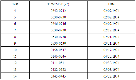
In the Table 1 we can see the series of INEL field experiments.

Table 1. Information about the INEL experiments

The INEL low wind speed diffusion experiments were accomplished in a flat and uniform terrain. The pollutant SF₆ was collected in arcs of 100, 200 and 400 m of the emission point at the height of 0.76 m above of the ground. The pollutant was released of a height of 1.5 m above of the ground-level. The wind in 2 m was obtained of the experiment. The roughness length for the INEL experiments was of 0.005 m.

The Monin-Obukhov length, friction velocity and height of the PBL were not measured in the INEL experiments, but were calculated from the empirical formulations.

The Monin-Obukhov length was calculated utilizing the following relation [14]

The friction velocity is calculated as [15]

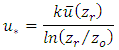where (reference height).

To calculate h we use the following expression [16]

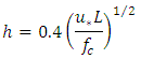where h is the stable turbulent PBL height.

3. Methods

To describe the meandering phenomenon behaviour and to capture the strong horizontal directional variations of the wind, there were accomplished simulations with WRF model in the INEL region, where the contaminant release experiments were performed (Table 1). The potential temperature profiles and heat fluxes generated by WRF model were utilized to run the LES-PALM model [17]. The horizontal wind field simulated by LES-PALM model was used to run the dispersion model based in the solution of the advection-diffusion equation.

In order to run the WRF model and provide meteorological inputs (heat fluxes and potential temperature), there were used reanalysis data of the NCEP/NCAR. The coupling between the numerical models considered 3 nested grids, being the data of the domain 3 selected to run the LES-PALM model (Figure 1). The Planetary Boundary Layer (PBL) parameterization used in WRF model was Mellor-Yamada Nakanishi Niino Scheme ([18], [19]).

Figure 1. The grids configuration used in the WRF model. d01, d02 and d03 are the WRF model domains

The present investigation employs the simplified form of the advection-diffusion equation written as [20]

(1)

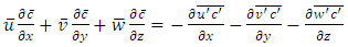
where represents the mean concentration of a passive contaminant; and represent the mean wind components ; and the terms and represent the concentration turbulent fluxes in x, y and z directions, respectively.

In order to solve the turbulence closure problem, it is used the hypothesis of gradient transport (K theory) [21] as following

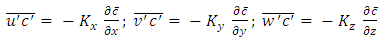(2)

where and are the eddy diffusivities along x, y and z directions, respectively. Replacing Equation (2) in Equation (1) is obtained the parameterized advection-diffusion equation [22]

(3)

where the terms on the left side are the advective transport and the terms on the right side are the diffusive transport. The boundary conditions for Equation (3) are

(4)

The source condition is

(5)

where is the emission rate, h is the PBL height, is the source height, and are the limits far from the source in x and y directions, respectively, and is the Dirac delta function. The horizontal mean wind components u and v are provided by

(6)

and

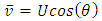(7)

where is the horizontal wind speed and is the wind direction. Assuming the vertical mean wind component and the derivative as equal to zero [23] in Equation (3), the following equation is obtained

(8)

Applying the integral transform technique in the y variable [24], one can write the pollutant concentration as

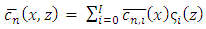
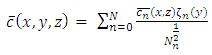(9)

where is given as

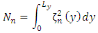and is a set of orthogonal eigenfunctions [25] with . Replacing Equation (9) in Equation (8) yields

(10)

Utilizing the following integral operator , remembering that (from the associate Sturm-Liouville problem) and using the orthogonality of the eigenfunctions, one can write the Equation (10) as

(11)

where

(12)

(13)

or in matrix form

(14)

Equation (11) is solved by the GILTT technique ([8], [26]). In this case, the two-dimensional concentration is given as

(15)

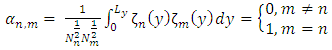
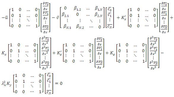
where is a set of orthogonal eigenfunctions with being a set of eigenvalues. Replacing Equation (15) in Equation (11), and following the same procedure adopted before, applying the integral operator using the ortogonality of eigenfunctions, Equation (11) is written in matrix form as

(16)

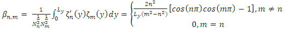
where is the column vector with components . The F matrix is given as and the G matrix is . The B, R and S matrices are written as

Applying the 3D-GILTT method in the source condition, one can write

(17)

where is the column vector with components

Applying an order reduction in Equation (16), we define new variables as and . By this procedure, the following equation in matrix form is obtained

(18)

where is given as and the H matrix is written as .

The Equation (18) is analytically solved by using the Laplace Transform Technique and the diagonalization [24]. Applying the Laplace Transform in the x variable, transforming x in s, we have

(19)

We can write H as , where D is the diagonal matrix of eigenvalues of the H matrix [27]; X and are the matrix and inverse matrix of eigenvectors, respectively [28]. After same algebraic manipulation, the solution of the Equation (19) is

(20)

where and , with the diagonal matrix . We can write the Equation (20) in matrix form

Finally, to determine , we need to solve the following linear system by applying the boundary conditions of the solution of the Equation (18)

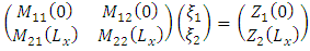Replacing the results of the Equation (20) in Equation (15) we obtain the solution of the two-dimensional problem (2D). Replacing the results of the problem 2D (Equation (15)) in Equation (9) we obtain the three-dimensional solution of the advection-diffusion equation.

Thus, employing stable PBL eddy diffusivities [10, 11] and the simulated horizontal wind field by the meteorological models in the above equations, the observed meandering effect in the dispersion of passive scalars can be described.

4. Results and Discussion

To simplify, only the results to the test 4 are shown (Figures 2, 3, 4 and 5). Figure 2 shows the vertical profile of potential temperature simulated by WRF model to the domain 3. This profile is typical of stable atmospheric conditions. We can observe an inversion layer close to the ground. Above this inversion, we can observe a neutral layer.

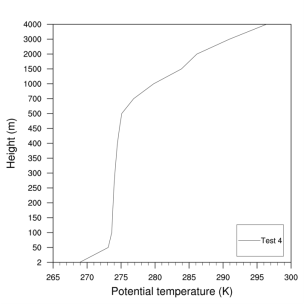Figure 2. Vertical profile of potential temperature simulated by WRF model

Figures 3 and 4 show the autocorrelations functions calculated based on the and wind components simulated by the LES model. It can be seen clearly in these figures the presence of negative lobes on the horizontal wind components. These negative lobes are striking features of the existence of the meandering phenomenon in atmospheric movements [2, 4]. Therefore, the strong negative lobes exhibited in figures show that the LES-PALM model is able to reproduce the principal characteristic of the wind meandering. The rate (in module) between the adjustment parameters of the wind component proposed by Frenkiel [29] is 2.220363 and the proposed by Moor et al [4] is 2.844219. The adjustment parameters of the wind component calculated from the Frenkiel [29] and Moor et al [4] are 2.491916 and 3.615198, respectively.

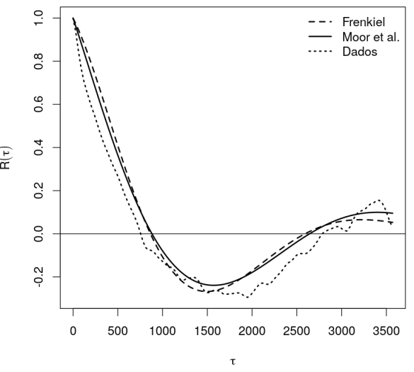Figure 3. Autocorrelation function calculated with the u wind component simulated by LES model

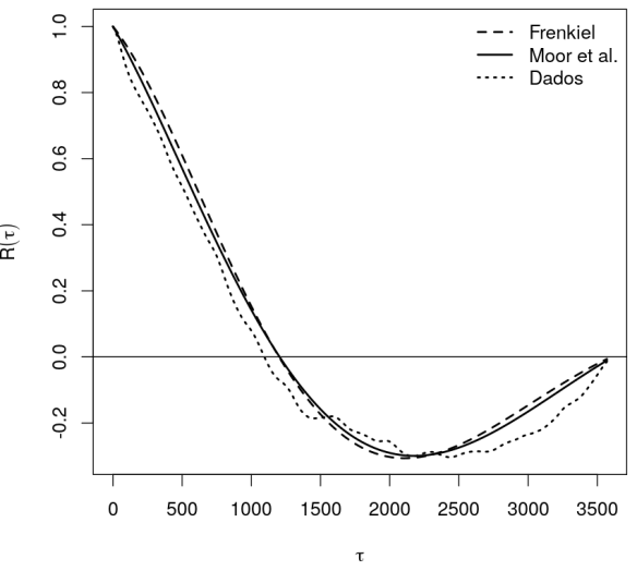Figure 4. Autocorrelation function calculated with the v wind component simulated by LES model

The contaminant concentration determined through the technique described in the Methods section is showed in the Figure 5 and one can see the meandering enhanced dispersion of the pollutants plume.

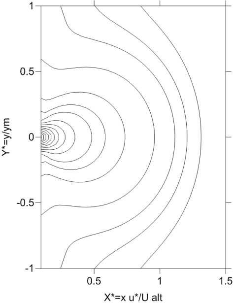Figure 5. The simulated pollutant plume by applying the 3D-GILTT technique in the advection-diffusion equation, is the friction velocity, U is the mean wind speed, is the planetary boundary layer height and ym is the maximum source distance in the y direction

Therefore, the hierarchy of the models above is able to simulate the large opening of the pollutants plume provoked by the action of the meandering phenomenon.

Figure 6 shows the scatter diagram of the observed and simulated concentrations using the algebraic eddy diffusivities and wind power law in stable conditions, considering and not considering, respectively, the wind meandering phenomenon. The scatter over the central line in Figure 6a is lesser than in the Figure 6b and hence we can see the importance of considering the wind meandering in air dispersion model.

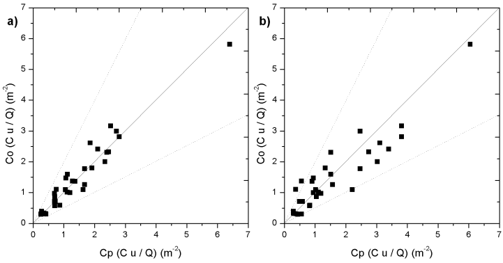Figure 6. Scatter diagram of the observed (co) and simulated (cp) concentration by 3D-GILTT method using wind power law and INEL experiment (a) the wind meandering is considered (b) the wind meandering is not considered

This reduced scattering of the simulated concentrations demonstrates that the dispersion model (3D-GILTT) considering the wind meandering is able to properly reproduce the observed contaminant concentrations.

Figure 7 shows the scatter diagram of the observed and simulated concentrations using algebraic eddy diffusivities and wind similarity law in stable conditions, considering and not considering, respectively, the wind meandering phenomenon. As in the Figure 6, better results are obtained when we consider the wind meandering phenomenon. If we compare both simulations with wind power and similarity law, better results are obtained when we consider the wind power law.

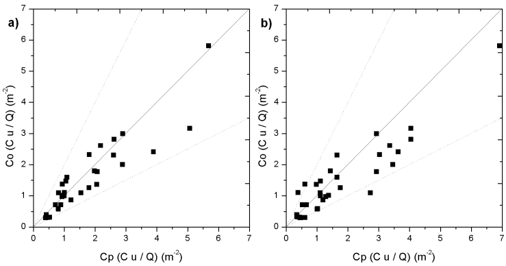Figure 7. Scatter diagram of the observed (co) and simulated (cp) concentration by 3D-GILTT method using wind similarity law and INEL experiment (a) the wind meandering is considered (b) the wind meandering is not considered

Table 2 lists the statistical performance [30] of the 3D-GILTT model in stable low wind conditions and also presents a comparison with other four different dispersion models. The simulated concentrations are in agreement with the observed concentrations. In this case, the Correlation coefficient (COR) and Factor of two (FA2) are near to one and the Normalized mean square error (NMSE), Fractional bias (FB) and Fractional standard deviation (FS) are near to zero. Furthermore, the 3D-GILTT approach using the meteorological modelling system presents results comparable or even better that one’s obtained by the other dispersion models. Two main conclusions are obtained, the first one is that better results are obtained when we consider the wind meandering phenomenon, independent if we use wind power or similarity law, and the second one is that better results are obtained when we use wind power law, independent if the wind meandering is considered or not considered.

Table 2. Statistical performance considering the 3D-GILTT model and other models for the INEL experiment

5. Conclusions

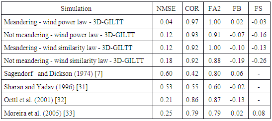
In low wind conditions to evaluate the contaminant concentration, the air dispersion models need to consider the meandering enhanced dispersion and also the turbulent diffusion processes. In this aspect, the turbulent parameterization plays a fundamental role in dispersion models that simulate the observed contaminant concentration. Therefore, the choice of an adequate parameterization allows a better description of the turbulent transport in the PBL.

In this study, an Eulerian air dispersion model based on the solution of the advection-diffusion equation (3D-GILTT), in which the simulated horizontal wind field is obtained from a meteorological modelling system (WRF and LES-PALM), is employed to simulate the contaminant concentration in low wind speed meandering situation. Its solution is obtained by applying the integral transform techniques. To represent the wind meandering effect, the horizontal wind generated from the LES-PALM is decomposed in the lateral and longitudinal directions. Concerning to the turbulent dispersion the Eulerian model uses eddy diffusivities, for stable condition, given by algebraic formulations that incorporate the physical characteristics of the energy-containing eddies. Furthermore, these eddy diffusivities describe the inhomogeneous character and the meandering effect associated to the PBL turbulence.

The horizontal velocity autocorrelation function shows the characteristics of the occurrence of the wind meandering phenomenon, presenting negative lobes with the ratio of the adjustment parameters greater than or equal to one. This fact points out that the LES-PALM model reproduces in a satisfactory way the relevant features associated with the wind meandering phenomenon.

The results of the simulated contaminant concentration by the Eulerian model (3D-GILTT) were compared with the observed concentrations in the INEL low wind experiments and other different turbulent diffusion models. In this aspect the results obtained by the 3D-GILTT incorporating the results of the meteorological modelling system, agree well with the experimental data, indicating that the model represents the diffusion processes correctly in low wind speed stable conditions. It is also possible to verify that 3D-GILTT results, utilizing the meandering dispersive effects, are better than those simulated by other dispersion models. Therefore, the new 3D-GILTT model incorporating the enhanced meandering dispersion, may be suitable for application in regulatory air pollution modelling.

ACKNOWLEDGEMENTS

This study was supported by CAPES (Coordenação de Aperfeiçoamento de Pessoal de Nível Superior).