-
Paper Information
- Paper Submission
-
Journal Information
- About This Journal
- Editorial Board
- Current Issue
- Archive
- Author Guidelines
- Contact Us
American Journal of Environmental Engineering
p-ISSN: 2166-4633 e-ISSN: 2166-465X
2016; 6(4): 110-122
doi:10.5923/j.ajee.20160604.02

Causal Linkage between Economic Growth, Financial Development, Trade Openness and CO2 Emissions in European Countries
 Abstract
 Reference
 Full-Text PDF
 Full-text HTML
Manel Ben Ayeche, Mounir Barhoumi, Mohamed Amine Hammas
Department of Economic Sciences, Faculty of Economic Sciences and Management of Sousse University of Sousse, Tunisia
Correspondence to: Manel Ben Ayeche, Department of Economic Sciences, Faculty of Economic Sciences and Management of Sousse University of Sousse, Tunisia.
| Email: |  |
Copyright © 2016 Scientific & Academic Publishing. All Rights Reserved.
This work is licensed under the Creative Commons Attribution International License (CC BY).
http://creativecommons.org/licenses/by/4.0/

In this paper, we examine the linkage between economic growth, financial development, trade openness and CO2 emissions. Empirically, we use the General Linear Model (GLM) for a panel data of 40 European countries over the period from 1985 to 2014. Our econometric methodology is based on the Cobb-Douglas production function. The empirical results show that there is evidence of bidirectional causality between economic growth and financial development, economic growth and trade openness, economic growth and CO2 emissions, financial development and trade openness and trade openness and CO2 emissions. From the linkage between economic growth and CO2, we verify the existence of the environmental Kuznets curve. Additionally, we validate the feedback hypothesis of the bidirectional causality between trade openness and financial development. Also, we identify the neutrality hypothesis between environmental degradation measured by CO2 emissions and financial development. Finally, we prove the bidirectional causality between economic growth and financial development and between economic growth and trade openness.
Keywords: Economic growth, Financial development, Trade openness, CO2 emissions, European countries, GLM
Cite this paper: Manel Ben Ayeche, Mounir Barhoumi, Mohamed Amine Hammas, Causal Linkage between Economic Growth, Financial Development, Trade Openness and CO2 Emissions in European Countries, American Journal of Environmental Engineering, Vol. 6 No. 4, 2016, pp. 110-122. doi: 10.5923/j.ajee.20160604.02.
Article Outline
1. Introduction
- The twentieth century was marked by the extraordinary success of the global economic system, with the industrialization and unprecedented technological progress has in the twentieth century size of its wealth more than twenty times. With these developments, the quality of life could be significantly improved for a large part of the population. The daily intake of calories per person indicates general upward trend in both developed and developing countries.Similarly, the proportion of people in poverty is illustrated by a general decline over the last fifty years. In a century, this extraordinary material enrichment has catalyzed an extremely rapid population growth, increasing global population of one billion people in more than six billion. The mortality rates have fallen dramatically, life expectancy has increased by more than two years on average, and infant mortality has been reduced to less than 60 per 1000 live births.At present, environmental concerns have taken center stage in national and international policy debates. Environmental problems are thus the concern of public opinion. They are now part of the political and economic choices.In addition, the international trend shows that various economies have resisted in attaining economic growth, financial development and trade openness exclusive of parallel observing a boost in CO2 emissions. Then, the relationship between economic growth, financial development, trade openness and environmental degradation is examined by various studies in the recent decades because the linkage between these factors has not been studied in detail recently, this research focuses on the bidirectional causality between all these economic aggregates.In this context, the main goal of our study is based on the question as follow: Why does our happiness decline as we become richer? Based on this question, the objective of this paper is to investigate empirically the bidirectional linkage causality between economic growth, financial development, trade openness and CO2 emissions. Methodologically, we use the General Linear Model (GLM) to estimate this causality from a panel data of 40 European countries during the period 1985 to 2014. The empirical results indicate that there is evidence of bidirectional causality between economic growth and financial development, economic growth and trade openness, economic growth and CO2 emissions, financial development and trade openness and trade openness and CO2 emissions. However, we remark the absence of the relationship between the financial development and CO2 emissions. These results are in conformity with the related literature.The rest of the paper is organized as Section 2 provides a review of related literature on the linkage between economic growth, financial development, trade openness and CO2 emissions. In Section 3, we describe the methodology. In section 4, we present the data used for empirical analysis. Section 5 offers the empirical results and a discussion of the study. Concluding remarks are presented in section 6.
2. Related Literature
- Several studies have been devoted to analyzing the existing of bidirectional causality between economic growth, financial development, trade openness and CO2 emissions.The analysis of the causality between economic growth and CO2 emissions is studied in much empirical research. This causality is based on the environmental Kuznets curve (EKC) hypothesis. This hypothesis provides that the relationship between economic growth and CO2 emissions is highly significant. In their studies, Grossman and Krueger (1991) [1] and Selden and Song (1994) [2] indicate that the causality between economic growth and CO2 emissions is positively significant. Their empirical results show that an increase in the economic growth augments the environmental degradation measured by the CO2 emissions.In addition, there are several books that focus on the existence of a large interaction between trade and the environment more precisely between trade liberalization and pollution (Anderson and Blackhurst, 1992 [3]; Etsy, 1994 [4]; Chichilnisky, 1994 [5]; Copeland and Taylor, 1994 [6]; Cole, 2000 [7]). In fact, it was verified that trade openness can, ceteris paribus; decrease pollution emissions that countries are facing a developed competitive pressure can be more solid in the use of resources. Others who have studied the practical implementation of trade liberalization through the GATT / WTO and assessed the level to which countries may limit imports of products dangerous to the environment. Nevertheless, Grossman and Krueger (1991) established the study of the correlation between trade and the environment that results distributed in three different effects. First, the scale effect is the probable augment into pollution resulting of the economic growth created by greater access to markets. Second, the technical effect submits to the evolution of production techniques which are likely to accompany the liberalization of trade. These can result from demand following the increase in income for the largest environmental regulations and better access for production technologies that respect the environment. Third, the composition effect refers to the changing composition of the economy and which has been occurring next the liberalization of trade that countries specialize more and more in activities that supply a comparative advantage. In fact, the composition effect is more interesting for the EKC and is the mechanism through which pollution haven would have an impact on the pollution.At the same time, these come when the continuous augmentation into revenue drive the change from capital intensive cumbersome industry activities to a service economy that produce less pollution. All in all, this phenomenon is named composition effect (Shafik, 1994) [8].As the activities of pollution in the developed countries are dealing with higher regulatory costs than poor countries, international trade and globalization boost the relocation of polluting industries to countries with the least regulated economic (Mani and Wheeler, 1998) [9]. This is referred to pollution haven hypothesis. This assumption can clarify, according to Mani and Wheeler (1998), reductions in the levels of deterioration of the environment in the developing countries and rising environmental degradation levels in the middle-income countries. During this time Andreoni & Levinson (2001) [10] reinforce the view that the EKC depends most directly upon the existence of scale economies in the elimination of pollution instead of the externalities, institutional political and the dynamics of growth.Besides, different argument that assists to clarify the EKC as the elasticity from demand for environmental quality. It is proved that the growth of GPD per capita leads to a further degradation of the environment in the first stages of economic development. But, income growth stimulates demand for a cleaner environment by expand the resource vacant to address versus pollution (World Bank, 1992) [11].Additionally, Roca (2003) [12] indicated that the willingness to pay for improvements in the quality of the environment increase a higher proportion than revenue, after encounter with some freeze of income. Furthermore, the quality of the environment probably will be regarded as a luxury good for certain levels of income. If the fundamental needs of people are achieved, their preoccupation for the environment rises (Dasgupta et al., 2002) [13].Likewise, when a community moves towards the realization of the social objectives, her institutions are reinforced to improving the regulatory framework and effectiveness of the control bodies which apply the existing legislation. Therefore individuals change their consumption habits towardsmore environmentally friendly products and the government pressure produce more strict environmental regulations (Dinda, 2004) [14]. As a result, Dinda (2004) show that the fragility of regulation in the developing countries led to a reduced capacity to uphold the established rules, that attracts multinational companies that develop highly polluting production processes.Azomahou et al. (2006) [15] show the existence of a linear relationship between economic growth and CO2 emissions. Lean and Smyth (2010) [16] and Saboori et al. (2012) [17] improve the presence of the inverted U-shaped relationship. The study developed by Friedl and Getzner (2003) [18] indicate an N-shaped relationship between economic growth and CO2 emissions. However, Richmond and Kaufmann (2006) [19] concluded a no causal relationship between economic growth and CO2 emissions.The causal relationship between economic growth and environmental can be shown by referring to the environmental Kuznets curve (EKC) hypothesis. The EKC explain the nexus between economic growth and environmental degradation since the 1990s. Then, Grossman and Krueger (1991) and Selden and Song (1994) developed empirical evidence which indicated that economic growth leads to a gradual degradation of the environment. Their impact is providing, in the initial stages and after a certain level of growth, the EKC hypothesis postulates that the link between economic growth and environmental degradation is non-linear and inverted-U shaped. This implies that economic growth is linked with an augment in CO2 emissions initially and declines it, once economy matures.The EKC hypothesis is studied by some researchers which found a conflicting result (Stern et al., 1996 [20]; Ekins, 1997 [21]; Heil and Selden, 1999 [22]; Managi and Jena, 2008 [23]; Fodha and Zaghdoud, 2010 [24]; Jaunky, 2010 [25]; Ozturk and Acaravci, 2010 [26]; Saboori et al., 2012).For country-specific study, Ang (2008) [27] for Malaysia, Soytas and Sari (2009) [28] for Turkey, Fodha and Zaghdoud (2010) for Tunisia, Ghosh (2010) [29], succeed in finding bidirectional causality between economic growth and CO2 emissions. But, Ang (2007) [30] for France, Jalil and Mahmud (2009) [31] for China, Nasir and Rehman (2011) [32] for Pakistan, and Saboori et al. (2012) for Malaysia succeed in finding an inverted-U shaped curve between economic growth and CO2 emissions. For multi-country study, Tsai (1994) [33] for 62 countries, Apergis and Payne (2009) [34] for 6 Central American countries and Omri (2013) [35] for 12 MENA countries concluded in their results an inverted-U shaped curve between economic growth and CO2 emissions. Also, the methodology employed in all these study is based on Granger causality. However, the relationship between economic growth and CO2 emissions is not found by Richmond and Kaufmann (2006) for panel of 36 countries, Halicioglu (2009) [36] for turkey, Ozturk and Acaravci (2010) for Turkey; Jaunky (2010) for 36 high-income countries, and Menyah and Wolde-Rufael (2010) [37] for South Africa.The importance of CO2 emissions in the environmental protection and their implication in all economic and financial sectors motivated some studies to integrate potential indicators to test the EKC hypothesis. Then, CO2 emissions are related to trade openness by Halicioglu (2009), Nasir and Rehman (2011), Shahbaz et al. (2013) [38], Omri et al. (2014) [39] and Omri et al. (2015) [40], to urbanization by Zhang and Cheng (2009) [41], Hossain (2011) [42], Sharma (2011) [43], Omri et al. (2014) and Omri et al. (2015), to financial development by Tamazian et al. (2009) [44], Tamazian and Rao (2010) [45], Yuxiang and Chen (2010) [46], Ozturk and Acaravci (2013) [47], Omri et al. (2014) and Omri et al. (2015).In fact, in case of the link between CO2 emissions and trade openness, Halicioglu (2009) examine how trade openness can explore the relationship between economic growth, CO2 emissions and energy consumption in Turkey. Their empirical results indicate that trade openness are one of the main determinants to economic growth while income increase the level of CO2 emissions. For Chinese provinces, Chen (2009) [48] concluded that industrial sector's development is linked with an augment of CO2 emissions due to energy consumption. By using ADF unit root test and co integration test, Nasir and Rehman (2001) studied EKC in Pakistan and indicated a positive effect of trade openness on CO2 emissions. However, Shahbaz et al. (2012) [49] show that trade openness reduces CO2 emissions. Moreover, Tiwari et al. (2013) [50] proved that trade openness increase environmental degradation in case of India. For the relationship between CO2 and all others economic and financial aggregates, Tamazian et al. (2009) examine the effect of other potential contributors to CO2 emissions such as economic, institutional, and financial indicators. In their study, Tamazian et al. (2009) investigated the effect of financial development on CO2 emissions in case of Brazil, Russia, India, China, Untied States and Japan. Furthermore, Tamazian and Rao (2010) studied the impact of institutions on CO2 emissions. Their empirical results indicated that economic development, trade openness, financial development and institution shave an important role to control the environment degradation while supporting the presence of Environmental Kuznets Curve hypothesis. Yuxiang and Chen (2010) prove that financial sector polices in China enables the firms to use advanced technology which reduceCO2 emissions and increase domestic production.Third strand deals with country case studies, for example in case of United States, Soytas et al. (2007) [51] examined the dynamic link betweenCO2 emissions, income and energy consumption. Their empirical results indicated that environmental degradation Granger causes income and energy consumption which contributes to CO2 emissions. Similar evidence was developed by Ang (2007, 2008) in France and Malaysia. The results showed that economic growth Granger causes energy consumption and CO2 emissions in two countries; France and Malaysia, unidirectional causality are found running from economic growth to energy consumption. From case of Tunisia, Chebbi (2010) [52] examine the causal relationship between energy consumption, income and CO2 emissions. The empirical results showed that energy consumption stimulates economic growth which Granger causes CO2 emissions. Ghosh (2009) uses Indian data to study the causal relationship between income and CO2 emissions by incorporating investment and employment as additional determinants of carbon emissions but the results show the absence of causality between income and CO2 emissions. In addition, Chang (2010) [53] applied multivariate causality test for Chinese data to investigate the causal linkage between economic growth, energy consumption and CO2 emissions. The results of the study indicated that economic growth Granger causes energy consumption that leads to carbon emissions.Based in all studies listed previously, our paper is addressed to investigate the causal relationship between economic growth, financial development, trade openness and CO2 emissions. Then, we use some additional determinants, as FDI, energy consumption, inflation, urbanization and capital stocks, which can play an important role to determinate this causal linkage. The empirical evidence is formed from panel data composed by 40 European countries during the period from 1985 to 2014. The econometric methodology is based on the utilization of the Cobb-Douglas production function which is estimated by the General Linear Model.
3. Econometric Methodology
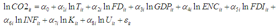
- To examine the linkages between economic growth, CO2 emissions, financial development, and trade openness, in European countries, we refer to the Cobb-Douglas production function. In this function, we explain the gross domestic product per capita (GDP) by tow economic aggregates; depends on capital and labor force. In addition, the economic growth measured by the GDP per capita depends also on financial development (FD), trade openness (T), foreign direct investment (FDI) and CO2 emissions (CO2). In this paper, we refer to the Cobb-Douglas production function. Then, we use four equations, as follow:
 | (1) |
 | (2) |
 | (3) |
 | (4) |
 is the constant.
  is the error term.
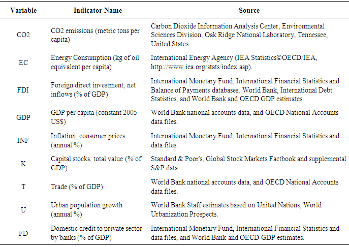
  are the estimated coefficients of all independent variables which j = 1, …, 8. The subscript i=1,…,40 denotes the country. The subscript t = 1, …,30 denotes the time period. Table 1 summarizes all variables used in this paper.In the equation (1), we examine the impact of the financial development, the trade openness, the CO2 emission per capita, the energy consumptions, the foreign direct investment, the inflation rate, the capital stock, and the urbanization rate on economic growth (Ang, 2008; Menyah and Wolde-Rufael, 2010; Anwar and Sun, 2011 [54]; Omri et al., 2014; Omri et al., 2015). Then, in the second equation, we study the effect of the GDP, the trade openness, the CO2 emission per capita, the energy consumptions, the foreign direct investment, the inflation rate, the capital stock, and the urbanization rate on the financial development (Ahlin and Pang, 2008 [55]; Ozturk and Acaravci, 2013; Omri et al., 2014; Omri et al., 2015). The equation (3) report the reaction on the Trade openness to the financial development, the GDP, the CO2 emission per capita, the energy consumptions, the foreign direct investment, the inflation rate, the capital stock, and the urbanization rate (Ozturk and Acaravci, 2013; Belloumi, 2014 [56]; Omri et al., 2014). Based on Lotfalipour et al. (2010) [57], Hossain (2011), Sharma (2011), Saboori et al. (2012), Omri et al. (2014) and Omri et al. (2015), we use the equation (4) to test the impact of the Trade openness, the financial development, the GDP, the energy consumptions, the foreign direct investment, the inflation rate, the capital stock, and the urbanization rate on the CO2 emissions.To estimate the above equations, we use the general linear model (GLM) in the case of panel data.
|
4. Data
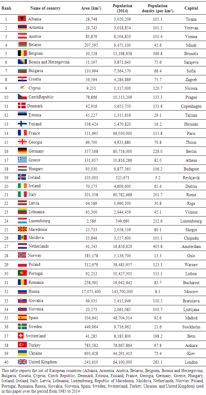
- This paper studies the relationship between four economic aggregates (Economic growth, financial development, trade, and CO2 emissions) in the European region over the period from 1985 to 2014. We use yearly panel data. The sample is formed by 40 European countries (Albania, Armenia, Austria, Belarus, Belgium, Bosnia and Herzegovina, Bulgaria, Croatia, Cyprus, Czech Republic, Denmark, Estonia, Finland, France, Georgia, Germany, Greece, Hungary, Iceland, Ireland, Italy, Latvia, Lithuania, Luxembourg, Republic of Macedonia, Moldova, Netherlands, Norway, Poland, Portugal, Romania, Russia, Slovakia, Slovenia, Spain, Sweden, Switzerland, Turkey, Ukraine, and United Kingdom). We present in Table 2 the list of the European countries used in this study.
|
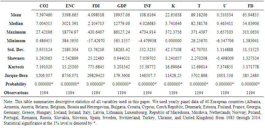 | Table 3. Descriptive statistics |
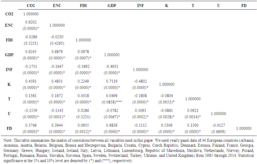 | Table 4. Matrix of Pearson correlation |
|
5. Results
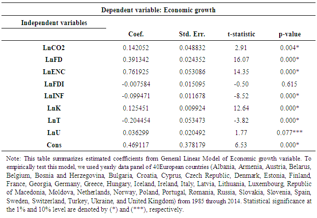
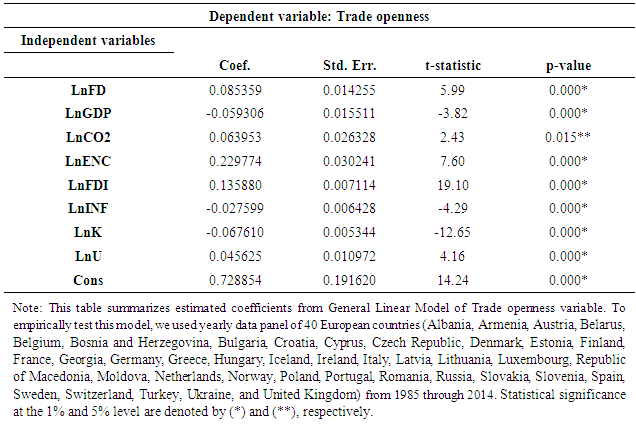
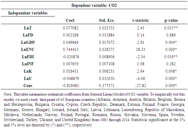
- We begin our empirical results by the presentation of the estimation coefficients of the equation (1). In this equation, we examine the degree of influence of the financial development, the trade openness, the CO2 emissions, the energy consumptions, the foreign direct investment, the inflation rate, the capital stock, and the urbanization rate on the economic growth. The estimation results of equation (1) are reported in table 6.
|
|
|
|
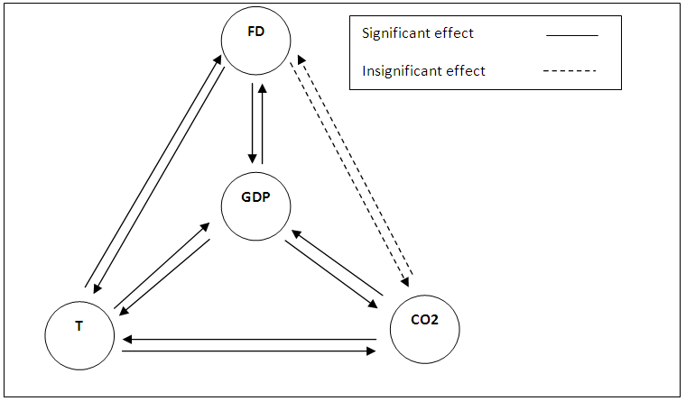 | Figure 1. The linkages between economic growth, financial development, trade openness and CO2 emissions |
6. Conclusions
- In this paper, we examine the relationship between economic growth, financial development, trade openness and CO2 emissions. Empirically, we use a General Linear Model from a panel data composed by 40 European countries over the period 1985-2014. The objective of our study is to test the linkages between economic growth, financial development, trade openness and CO2 emissions by employing four structural equations that allow one to observe the impact of (i) CO2 emissions, financial development, trade openness and other variables on economic growth; (ii) economic growth, CO2, trade openness and other variables on financial development; (iii) financial development, economic growth, CO2 emissions and other variables on trade openness; and (iv) trade openness, financial development, economic growth and other variables on CO2 emissions.The main result of our study show evidence of bidirectional linkage between economic growth and CO2 emissions, economic growth and financial development, economic growth and trade openness, financial development and trade openness, and trade openness and CO2 emissions. However, we find an absence of the significance linkage between financial development and CO2 emissions in the case of the Europeans countries. Figure 1 reports the existing linkage between the four fundamental economic aggregates. The empirical finding of this study, show that the economic growth and the environmental degradations are positively correlated. The economic growth predicts a positive relationship with the CO2 emissions. Additionally, the economic growth promotes the financial development in the case of Euro zone. But, the economic growth can prevent the trade openness. The increase in financial development can increased the trade openness. Finally, we show a positive relationship between CO2 emission and trade openness. The results presented in this paper conform with the related literature.