-
Paper Information
- Next Paper
- Previous Paper
- Paper Submission
-
Journal Information
- About This Journal
- Editorial Board
- Current Issue
- Archive
- Author Guidelines
- Contact Us
American Journal of Environmental Engineering
p-ISSN: 2166-4633 e-ISSN: 2166-465X
2016; 6(2): 52-61
doi:10.5923/j.ajee.20160602.03

Modeling the Relation between Carbon Dioxide Emissions and Sea Level Rise for the Determination of Future (2100) Sea Level
 Abstract
 Reference
 Full-Text PDF
 Full-text HTML
1Department of Chemical Engineering, King Abdulaziz University, Rabigh, Saudi Arabia
2Department of Chemical Engineering, University of Southern California, Los Angeles, USA
Correspondence to: Hisham A. Maddah , Department of Chemical Engineering, King Abdulaziz University, Rabigh, Saudi Arabia.
| Email: |  |
Copyright © 2016 Scientific & Academic Publishing. All Rights Reserved.
This work is licensed under the Creative Commons Attribution International License (CC BY).
http://creativecommons.org/licenses/by/4.0/

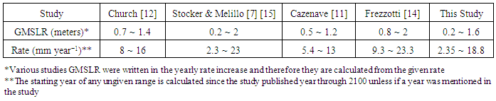
This paper confirms that there is a strong relationship between global warming (CO2 emissions) and global mean sea level rise (GMSLR). We discussed some statistics and facts regarding to the history of CO2 emissions as well as the present situation and how do CO2 emissions play a key role in controlling Earth’s temperature. A decent portion of this study covered valuable literature information on the topic of GMSLR which is a major global problem that resulted from climate change. The main two reasons for GMSLR are melting of glaciers or ice sheets and thermal expansion of seawater. Submerging coastal cities, soils’ contamination and damaging animals’ habitats are various consequences of GMSLR. The essential part in our study is to find the exact range of GMSLR by 2100 via establishing a model that is based on comparing previous increases in CO2 emissions with changes in sea level rise at the same time. Two scenarios of CO2 emissions are considered and they are the minimum (RCP2.6) and the maximum (RCP8.5) according to IPCC. Future GMSLR data for both scenarios are calculated for the overall rise, individual oceans and different seas. Rise in Earth’s temperature and radiative forcing (heat flux) are investigated for both scenarios and a proportional correlation is approved. Moreover, temperature anomalies data are obtained to identify the future differences between both scenarios. Results showed that, by 2100, GMSLR would be between 0.2-1.6 meters with an annual increase rate of 2.35-18.8 mm/yr. It is worth mentioning that our calculations confirmed that by the end of 2015 the total rise in temperature, since 1880, was around 0.85°C. However, by the end of the twenty-first century, the total change in heat flux would be about 2.5 and 8 W/m2 for RCP2.6 and RCP8.5 scenarios, respectively, and the accumulated temperature rise, since 1880, would be between 1.22°C and 4°C.
Keywords: Ocean, Sea level rise, Climate change, Global warming, CO2 emissions, Modeling, Temperature anomaly, Radiative forcing, Earth’s heat flux, Future, 2100
Cite this paper: Hisham A. Maddah , Modeling the Relation between Carbon Dioxide Emissions and Sea Level Rise for the Determination of Future (2100) Sea Level, American Journal of Environmental Engineering, Vol. 6 No. 2, 2016, pp. 52-61. doi: 10.5923/j.ajee.20160602.03.
Article Outline
1. Introduction
- Carbon dioxide (CO2) constitutes only about 0.04% of air; but it plays a crucial role in controlling Earth’s average temperature. However, bulk air elements like nitrogen (N2) or oxygen (O2) are not capable of absorbing heat radiation. The opposite is true for water vapours (clouds) which are able to absorb 75% of the sun’s radiation. Yet, clouds cannot control planet overall temperature since that water vapours depend on air circulation and they condense without being able to keep Earth’s temperature at lower rates. On the other hand, CO2 gas is independent of the previous parameters and has a strong tendency to absorb sun energy which reduces Earth’s surface heat radiation to space. Higher CO2 leads to higher temperature and humidity in the atmosphere; more or extra temperature will be added from having more water vapours. Thus, CO2 acts as a control knob that controls the amount of water vapours and clouds in Earth’s atmosphere [1-3]. There is a strong correlation between CO2 emissions and rise in temperatures. Although correlation does not equal causation, scientists believe that greenhouse gases are driving the glob’s temperature higher especially after observing some indications like the increase in ice melting rate, deep ocean heat and sea level rise [6]. According to the Intergovernmental Panel on Climate Change (IPCC), global average temperatures on both land and ocean surfaces have increased about 0.85°C (1.53°F) from 1880 to 2012. Global records of NASA and NCDC corporations revealed that the decade between 2000 and 2009 is the hottest decade, with an average temperature of 12.2°C, since the beginning of modern technology about a century ago. Further, the warmest 30-year period was from 1993 to 2012 since 1400 years and global records indicate that earth atmosphere is getting warmer than before [7].Global warming may be interpreted in various environmental signs such as dense clouds, massive recurring floods, powerful snowstorms or even extreme drought periods. Higher Earth’s temperature enhances ocean evaporation rate which yield to heavier precipitation. For example, total precipitation between 1958 and 2007 in United States increased by three folds and resulted in critical weather conditions like flash floods. Early studies showed that flood fatalities in United States had a significant number compared to previous statistics that prior to 1958 because of the change in weather conditions. By 2090, CO2 emissions will increase precipitation events in United States by an average of 36%. Engineering solutions and strict plans are mandatory in order to avoid such a calamity in the near future [8]. Further, other problems that are associated with global warming include sea level rise, ice and snow melting, higher oceans acidity, extreme weather conditions and threats to human health [7]. Extreme weather conditions involve increase in extreme high temperatures or decreases in extreme low temperatures and these situations are related to the fact that states every 1°C rise results in adding 7% of moisture to the atmosphere. Higher moisture means more intense precipitation events will occur. In addition, moisturized warm atmosphere is an ideal situation for powerful hurricanes. Astoundingly, climate change plays a key role in present extinctions and distributions of wildlife animals and plants. Extreme drought environments could be linked to current changes in atmospheric circulation. Potential researchers should consider conducting a more concisely comparative study between temperature and precipitation data which will allow us to determine the exact impact of global warming on weather conditions [9] [10].Unfortunately, cutting CO2 emissions is not a viable solution to global warming dilemma anymore. This is because greenhouse gases characterize by the ability to stay in the atmosphere for a long time. Ocean’s response to higher greenhouse gases takes longer time than lands and therefore global warming will continue for several decades. Hundreds of years will pass before noticing a decrease in CO2 emissions or global temperature [7].
2. Global Mean Sea Level Rise
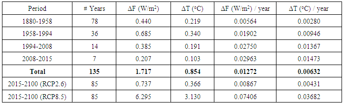
- One of the main consequences of global warming is the increase in the global mean sea level rise (GMSLR). Rate of the rise was modest between 1900 and 1930 since then the rate, over the past 50 years, increased to 1.8 ± 0.3 mm year−1. For the period 1993-2007, earlier studies reported rates of 2.85 ± 0.35 mm year−1 and 3.3 ± 0.4 mm year−1 in climate-related contributions and altimetry-based sea level rise, respectively, which indicates that sea level rise is mostly caused by global warming, Table 1. Even though data on thermal expansion indicate a less increase to the range 2003-2007, sea level has continued to rise. It was observed that around 30% of the rise is due to ocean thermal expansion and 55% resulted from land ice melt. Severe acceleration in melting rates and ice mass loss during the past five years increased the contribution of land ice melt from 55% to 80%. Further, there are some expectations of an additional 320% GMSLR caused by thermal expansion by 2100. An acceleration in the rate of sea level rise of 0.013 ± 0.006 mm year−2 was recorded between 1870 and 2004 [11].
|

2.1. Glaciers and Ice Sheets
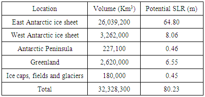
- Climate change predictions regarding to ice, snow and glaciers melting rates are shocking. Snow in the Northern Hemisphere plus Greenland and Arctic region have been melting for a long time and melting rate is expected to increase over the next century [7]. About 15% decrease in the extent of annually averaged Arctic sea ice is caused by 1.1°C (2°F) of warming. Snow seasons are expected to be shorter and melting starting sooner. Warmer temperatures advance ocean expansion and ice sheets, snow and glaciers melting rates that would significantly contribute to the GMSLR [16].Total land glaciers on Earth are around 10% and melting these glaciers will result in a potential sea level rise of 66 meters. Approximately 99% of this rise is accounted for the volume of polar ice sheets including Greenland and the Antarctic which are the most vulnerable locations for today’s climate change. The extent of the surface melt area of Greenland ice sheets (12% of total glaciers) increased over the last 30 years with an increase rate of −263 ± 30 Gt year−1 between 2005 and 2010 and that is equivalent to a sea level rise of 0.72 ± 0.08 mm year−1. Over the same interval 2005-2010, Antarctic ice sheets (87% of total glaciers) had an ice loss of −81 ± 37 Gt year−1. Although mountain areas contain less than 1% of the total glaciers, a total ice loss of −259 ± 28 Gt year−1 that is equivalent to a sea level rise of 0.71 ± 0.08 mm year−1 was recorded in the period 2003-2009. The overall contribution of glaciers and ice sheets in sea level rise is about 60% in the period 2003-2009. Sea level rise projections by the end of 2100 have been proposed to be between few decimetres and 2 meters [14].The present status of glaciers shows retreat and mass loss because of the higher air and surface ocean temperatures that is directly or indirectly caused by the human impact. Several studies confirmed that present ice loss from mountain glaciers, Greenland and West Antarctica is associated with global warming; and if the ice loss continued, sea level rise would be between 0.8-2 meters by the end of 2100 [14]. Another work showed that if total amount of ice sheets in Greenland and West Antarctica melted a sea level rise of 7 meters and 3-5 meters would happen, respectively. A significant elevation decrease in glaciers was found over 1992-2003 which confirmed the widespread ice mass loss in West Antarctica whereas East Antarctica was found stable. Since 1970, most of glaciers around the world have been retreating and thinning with obvious acceleration; glaciers contribution in sea level rise in 2006 was 1.1 ± 0.24 mm year−1. Sources of land waters (freshwaters) include rivers, lakes, snow pack, wetlands and aquifers are in continues exchange with atmosphere and oceans through evaporation, precipitation and rivers runoff [11]. Different studies suggested that the imbalance ice melting of Greenland and Antarctica contributes in sea level rise by 0.2-0.6 mm year−1. Moreover, melting of land glaciers enhances the rise by 0.2-0.4 mm year−1 [20].20,000 years ago, global sea level was about 125 meters below the current sea level. Recent warm atmosphere boosted melting rates of Antarctic ice sheets causing sea level to rise reversibly. Since the “Little Ice Age” in the nineteenth century, sea level has been rising about 1-2 mm year−1 due to the reduction in volume of ice caps and mountain glaciers as well as the thermal expansion of ocean water. Continues global warming will decrease Iceland’s glaciers 40% by 2100 and nearly disappear by 2200. Antarctic and Greenland ice sheets constitute most of the current global land ice mass; sea level would rise about 80 meters if complete melting of ice sheets occurred. However, melting of all other glaciers would contribute to the rise by only 0.5 meter. Melting of ice sheets at different locations contributes differently to the sea level rise. In other words, melting ice sheets of Greenland and West Antarctic would rise the sea level by 6.6 and 8 meters, respectively. Table 2 shows the estimated maximum sea level rises from total melting of glaciers in different locations [17] [18].
|
2.2. Thermal Expansion and Salinity
- Alterations in ocean water temperature and salinity change water density and therefore rising water occupied volume which lead to an increase in oceans level. Currently, the Earth is struggling with an imbalance state of energy since that oceans are able to store 85% of excess heat from climate change. Statistics confirmed the previous fact by showing that the amount of heat stored in oceans (16 x 1022 J), during the last 40 years, is approximately 15 times greater than heat stored on continents and approximately 20 times than that stored in the atmosphere. The mean thermal expansion trend over 1955-2001 is 0.4 ± 0.01 mm year−1 and 0.3 ± 0.01 mm year−1 followed by expansion rates range from −0.5 ± 0.5 mm year−1 over 2003-2007 to +0.4 ± 0.1 mm year−1 over 2004-2007 and +0.8 ± 0.8 mm year−1 over 2004–2007 [11]. The third IPCC report adopts that the largest contribution to the twentieth century GMSLR of 0.7 mm year−1 arises from thermal expansion while oceans warmed since the 1950 [20]. Regarding to salinity factor, redistribution of salinity by ocean circulations has an impact on regional scales, but it does not have an effect on the overall GMSLR [11]. Figure 1 shows the effect of thermal expansion on GMSLR from various previous studies simulations [21].
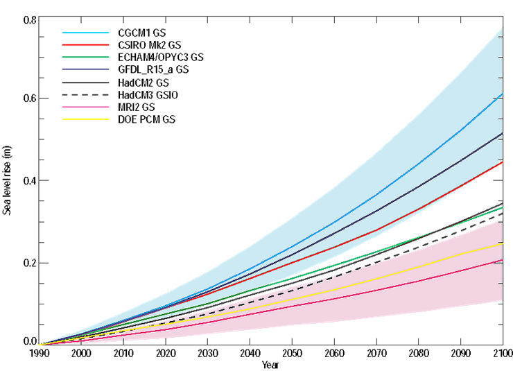 | Figure 1. Various simulations of GMSLR from thermal expansion [21] |
2.3. Consequences
- As mentioned previously, Earth’s surface temperature increases when high concentrations of greenhouse gases are released to the atmosphere; this explains the direct correlation between GMSLR and global warming. Sea level rise is caused by thermal expansion of water and melting of ice sheets and glaciers. Studying the outlook of sea levels during the far past have been helpful in understanding and forecasting the potential of GMSLR. For instance, recent studies found that Pliocene epoch (5.3-2.6 million years ago) sea levels were about 100 feet higher than they are today since global temperatures were between 3-4°C warmer [23].To understand long-term effects of global warming, four different scenarios of long-term CO2 emissions were developed by the IPCC, shown in Figure 2, using various assumptions regarding to future economic, technological and environmental conditions. Global average temperature is expected to double by 2100; meaning that worldwide average temperature would be between 0.27-4.7°C (0.5-8.6°F) and United States temperature between 1.6-6.66°C (3-12°F) [7]. Another source mentioned that by 2100, the change in global surface temperature was found by the IPCC models to be at a maximum value of 4.1°C (RCP8.5) and a minimum value of 1°C (RCP2.6) where 8.5 and 2.6 constants refer to expected Earth’s radiative forcing or heat flux values by 2100 [22]. However, land temperatures are expected to increase quickly compared to ocean temperatures [7]. Previous models showed that heavy precipitation would likely to occur in different regions with uneven water distributions. United States northern areas would become wetter while southern areas would be drier [15].
 | Figure 2. Projected greenhouse gas concentrations for four different CO2 emissions models [22] |
3. Methodology and Data
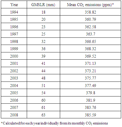
- Sea level rise calculations are initiated by simply comparing between two sets of data. Mean CO2 emissions data, extracted from NASA database and shown in Table 3 [24], in the period 1994-2008 are compared with mean sea level rise data, obtained from global mean sea level satellite altimetry between January 1993 and December 2008 [11], over the same 15-year interval in order to establish our model for further calculations. The model is established by comparing the yearly increments in both CO2 emissions and sea level rise. Combining both datasets (1994-2008) of CO2 emissions and sea level rise together allowed us to calculate future estimations with respect to GMSLR. Our goal is to obtain the maximum and the minimum values of GMSLR in the twenty-first century (2000-2100) by using IPCC RCP8.5 (maximum) and RCP2.6 (minimum) CO2 emissions scenarios shown in Figure 2. Also, a comparison between forecasted CO2 emissions and GMSLR would reveal the strong relation between both parameters. The effect of GMSLR on different oceans and seas is determined by utilizing information of seas surface areas with an assumption that we have same elevations at different locations [25].
|
 | (1) |
 | (2) |
4. Results and Discussions
- Figure 3 shows the proportionality in the relation between GMSLR and CO2 emissions in the period 1994-2008. Whenever there is an increase in CO2 emissions (global warming), there is also a parallel increase in GMSLR. Figure 4 illustrates the modeling data that is used in our study. The behaviour of both CO2 emissions and GMSLR is almost the same along the past decade. Minor inconsistencies between both lines in Figure 4 are observed, e.g. the case of year 2007 and 2008, but the overall correlation between the rise in CO2 emissions and the increase in GMSLR is clearly proportional. Thus, the two studied scenarios (RCP2.6 and RCP8.5) gave us results that, of course, similar to the model that we utilized in our calculations. Figure 5 confirms the relation between both variables, CO2 and GMSLR, and it states that GMSLR would be at a minimum and a maximum level of 0.2 and 1.6 meters, respectively, by 2100. Further, CO2 emissions would be between 460-1300 ppm by the end of the twenty-first century.
 | Figure 3. Correlation between GMSLR and CO2 emissions during the period (1994-2008) |
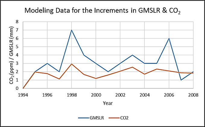 | Figure 4. Modeling data for GMSLR and CO2 emissions during the period (1994-2008) |
 | Figure 5. Forecasted relation between GMSLR and CO2 emissions during the period (2000-2100) |
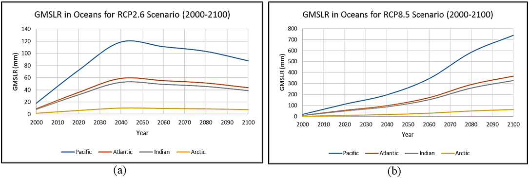 | Figure 6. Comparison between the projected GMSLR in different oceans for the two CO2 emissions scenarios (2000-2100) |
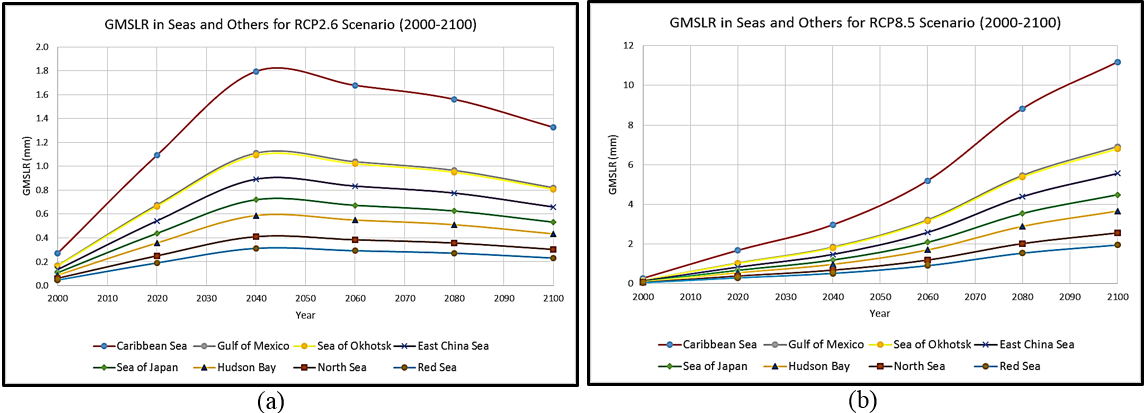 | Figure 7. Comparison between the projected GMSLR in different seas for the two CO2 emissions scenarios (2000-2100) |
|
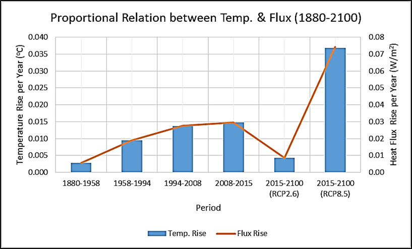 | Figure 8. The relation between temperature rise and CO2 emissions since the past until both future scenarios (1880-2100) |
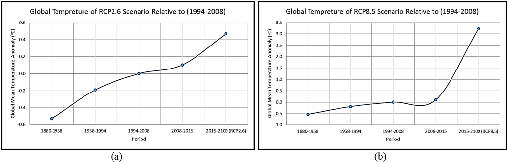 | Figure 9. Comparison between global temperature anomalies relative to 1994-2008 in both CO2 emissions scenarios (1880-2100) |
|
5. Conclusions
- Modeling the relation between global warming and GMSLR is achieved successfully by looking at previous CO2 emissions and sea levels data. IPCC minimum (RCP2.6) and maximum (RCP8.5) scenarios are necessary to determine our future expectations on GMSLR. Sea level rise issue will continue as long as humans keep burning fossil fuels and generating undesired amounts of greenhouse gasses. Oceans have higher tendency for thermal expansion in higher temperature atmosphere and therefore water volume increases. Additionally, warmer Earth’s surface yield to higher melting rates of both glaciers and ice sheets in Greenland and Antarctic regions. Our results concluded that GMSLR will likely increase by an annual increase rate of 2.35-18.8 mm year−1 and that is equivalent to a rise of 0.2-1.6 meters in 2100. The calculated GMSLR range is compared with previous studies values that had almost similar range of what we have obtained. Another confirmation to our results is the determination of the total rise in temperature in the period 1880-2015 which is around 0.85°C and similar to literature data. However, accumulated temperature rise is expected to be between 1.22°C and 4°C by the end of the twenty-first century. The simple linear model provided an approximation to the GMSLR by 2100 as compared to previous studies. Our model may not apply to other studies because it is simplicity may show flaws in other cases. We had a special case in which a particular set of data was in agreement with previous works after using linear correlations. In fact, there are many other advanced studies with more complex models which showed more accurate results to the GMSLR. Our model is only an attempt to confirm, develop and enhance previous calculated GMSLR data in a simple way. Next generations should consider the highly negative impact of future sea level rise on society; hence, more complex and accurate models, advanced observations and coastal impact studies should remain a major area of future climate research.
ACKNOWLEDGEMENTS
- The author would like to thank the Saudi Arabian Cultural Mission (SACM) for supporting, funding and encouraging me to accomplish this work, without whom this research would not be possible.