Nagia Elghanduri
Chemical Engineering Department, University of Tripoli, Libya
Correspondence to: Nagia Elghanduri, Chemical Engineering Department, University of Tripoli, Libya.
| Email: |  |
Copyright © 2015 Scientific & Academic Publishing. All Rights Reserved.
Abstract
This paper presents a statistical analysis for tracer dispersion in turbulent flow within and over a permeable bed. The analysis is made for the concentration change spatially and temporally. The spatial and temporal statistical tests provided establishment for tracer migration with turbulent flow within and over permeable bed. The study includes statistical investigation for the effect of bed geometry, tracer location and injection duration on tracer dispersion through fully developed turbulent flow in detail. The temporal statistical analysis for the tracer distribution was computing for the variance. The second is for the spatial variance, where the skweness and the variance were estimated using previously published correlations. Compute the time variance, spatial variance and skweness. The input data for each case was the averaged concentration with time for different locations within each flow zone. The results were compared graphically. It is found that the spatial variance increases at the zone where it penetrates to, which indicate that there is a continuous tracer support from the source zone to the other one. Further, the free stream pulse injection results show that there is a higher rate exchange between the free stream and porous zone than that on the opposite situation. Furthermore, the time variance is higher at the sparse case compared with the dense case.
Keywords:
Skweness coefficient, Variance, Tracer dispersion, Porous bed, Turbulent flow, Statistical analysis, Pulse injection, Continuous injection
Cite this paper: Nagia Elghanduri, CFD Tracer Tracking within and over a Permeable Bed II: Statistical Analysis, American Journal of Environmental Engineering, Vol. 5 No. 3, 2015, pp. 72-78. doi: 10.5923/j.ajee.20150503.03.
1. Introduction
As well known, the turbulent flow through and over permeable bed causes flow heterogeneity in time and space. The spatial heterogeneity and temporal variability causes fluctuations in tracer concentration due to fluctuation in spreading rate. This causes difficulties to track a tracer or pollutant spread in this type of flow. However, the statistical analysis gives indication for the tracer dispersion and movement, and helps to quantify statistically its concentration. It is also identify the quality of the main flowing fluid in different locations. The statistical analysis has been widely used in tracer tracking. A number of statistical techniques have been developed such as [1] presented a statistical field data for a river. Thomson, 1990 proposed three dimensional stochastic model for the particle motion in high Reynolds number. In open channels, experimental studies have been analyzed statistically, such [4], [5], and [6]. Further, [7] presented statistical analysis for chemicals in rivers. However, none of these methods are based on exact detail flow data. Further, still there is no consensus in literature on the value of the intensity of concentration fluctuations (i.e. standard deviation of concentration divided by mean concentration). On the other hand, because the complexity and nonlinearity of turbulent flows prohibiting the exact calculation of concentration statistics directly from the governing equations ([2]). The Computational Fluid Dynamics (CFD) techniques helped to get a detailed data for tracer dispersion in open channels. This data can be averaged through the tested zones to estimate very close investigation to the real results. This technique is widely used in this area of study such as [3]. This paper includes statistical test for tracer movement within and over a permeable bed based on detailed tracer data. It is continuation to the detailed analysis presented in the previous paper “CFD Tracer tracking within and over a permeable bed for surface injection I: detail analysis” by the same author. The test is for the effect of bed porosity, injection location, and the type of injection. Two different bed porosities have been tested.
2. The Studied Cases
The studied cases are flumes with two flow zones; Porous Zone and flow zone over it called Free Stream Zone. The Porous Zone consists of rows of rods mounted horizontally at specified distances. The studied cases are two, with different bed porosities. The first case is called sparse case (spar30) with a sufficient space between the obstacle for turbulent vortices to form a complete eddies and flow returns laterally. The second case is the dense case (dens30) which characterized by having small gaps between the obstacles. This causes distinct recirculation vortices at the downstream side of each obstacle and with very shallow penetration of turbulence, which does not go beyond these vortices ([8]). The simulation was for fully developed turbulent flow within and over permeable bed. Large flumes were built to reach turbulent fully developed regions. Figure 2 shows schematic diagram for the columns and rows of the arranged rods bundle symbols for geometry and hydrodynamic characteristics of the simulated cases. The numerical simulation used Fluent within Ansys 12 software. The tracer tracked numerically with the flow using Discrete Phase Model (DPM). The tracer injection was over the whole vertical depth to the flow for initially tracer free zone (at t=0, no tracer exist) and tracked over testing time. Further, two injection periods were tested. One is for 0.1 sec, and the second was continuous. The resulted data were exported for different time intervals as an ascii files. A computer programs were built using Matlab Software to read the ascii files. These programs grid the data and scatter it over the whole tested flow zones. The data then averaged to overcome the flow heterogeneity due to turbulence and upscale the microscopic quantities. Ten different locations far from the source have been averaged. Averaging technique is well known technique and widely used to overcome the instantaneous values for turbulent flow variables. In this study, the data before used was averaged twice (double averaging). The first averaging was from center to center between two columns (vertically), then averaging over the flow height. 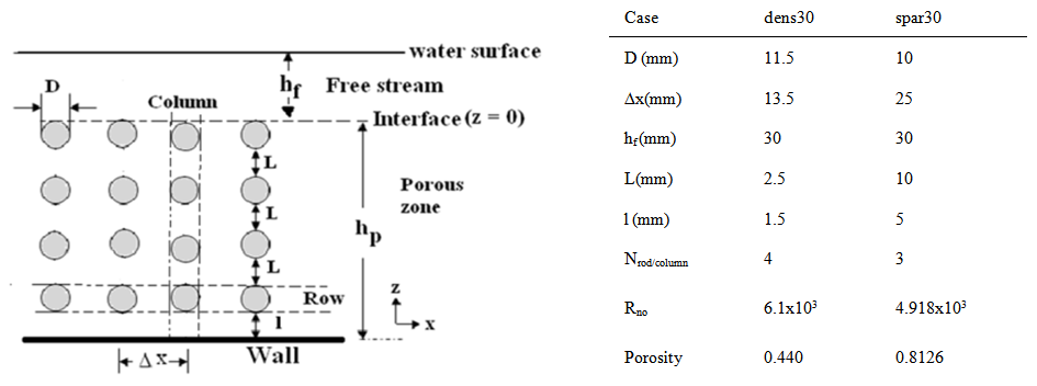 | Figure 1. Columns and rows of the arranged rods bundle symbols for geometry and hydrodynamic characteristics of the simulated cases |
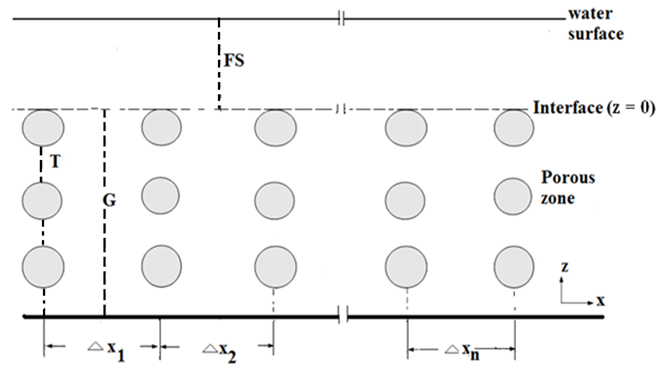 | Figure 2. Surface injection locations in the free stream (FS), and in the porous zone (T, and G) |
3. Theoretical Background
3.1. Tracer Distribution with Time
The time variance and skweness coefficient are important parameters in characterizing the shape of the concentration distribution. This type of analysis has been published previously in some literatures and expressed as the skweness coefficient such as [9], and [10]. The time variance: 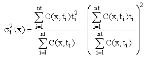 | (1) |
The definition of the skweness coefficient in time, for a given x-location is: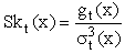 | (2) |
Where: gt(x) is and computed as:
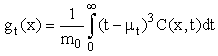 For a sample of C(x, ti) values recorded at time instances ti, i = 1, 2…, nt, i.e. for a set C(x, ti) the statistical moments can be evaluated as ([5]):
 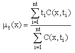 | (3) |
3.2. Tracer Distribution with Distance
Several studies for tracer tracking used distance variance analysis such as, [4], [5], and [6]. The spatial moment is defined as: 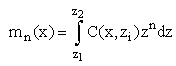 | (4) |
Where z1, and z2 are the height of the tested zone.The second spatial moment (m2(x)) is the spatial variance σz2(x), which can be evaluated as: 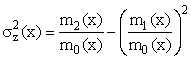 | (5) |
4. Results and Discussion
4.1. Tracer Distribution with Time
4.1.1. Pulse Injection
The results presented in this section are for surface pulse injection scenarios. Figure 3, and Figure 4 show the time variance and skewness coefficient respectively. These statistical values were computed at various x-locations (Figure 1) for both free stream, and the porous zone. It can be noticed that the time variance at the free stream injection is increasing with distance with the same pattern as that presented by [10]. Further, it has lower values compared to the other two porous zone injection scenarios. This is because the tracer at the free stream moves at higher speed compared to that at the porous zone. Furthermore, the tracer penetrates form the porous zone is continuous, and with faster rate at G-injection as the tracer source is closer to the free stream. However, far from the source the decrease in the time variance indicate a decrease in tracer migration to the other zone. On the other hand, at the dense case, a sharp decrease in the time variance values is noticed within the porous zone which is due to tracer low velocity. The curve for the dense case is not smooth because the tracer moving velocity is the same as that for the flow, which increases with bed height (profile shown in [8]) which is higher in the dense case.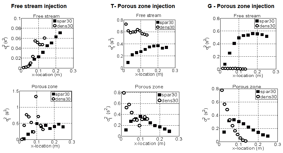 | Figure 3. The time variance coefficient for both spar30, and dens30 cases results from pulse three surface injection scenarios. The upper are for the tracer distribution at the free stream, and the lower are for the tracer distribution at the porous zone |
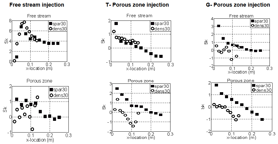 | Figure 4. The skweness coefficient for both spar30, and dens30 cases results from pulse three surface injection scenarios. The upper are for the tracer distribution at the free stream, and the lower are for the tracer distribution at the porous zone |
The skweness (Sk) coefficient for pulse injection (Figure 4) show a pulse pattern at the free stream as the tracer is injected for certain time. Further, the Sk coefficient is decreasing with the distance to the right side. However, a change in this pattern is shown far from the source zone at dens30 case, which is possibly due to the return of some penetrated tracer from the free stream. Furthermore, the pulse injection shows that there is higher rate of exchange between free stream and porous zone if the tracer is at the free stream, which is difficult to recognize at continuous injection.
4.1.2. Continuous Injection
The time variances for the three continuous injection scenarios are shown in Figure 6. From the figure it can be noticed the decrease in the time variance with x- coordinate for all injection source zones, with reasonably higher rate for the dense case. Further, the time variance is higher at the sparse compared with the dense case is due to the higher difference in velocities. Furthermore, the time variance values for the spars case are close at both free stream and porous zones for all injection scenarios. This is maybe due to the large bed porosity.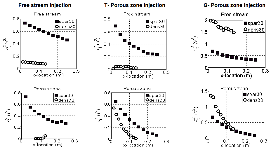 | Figure 5. The time variance for both spar30, and dens30 cases results from continuous surface injection scenario. The upper three are for the tracer distribution at the free stream, and the lower are for the tracer distribution at the porous zone |
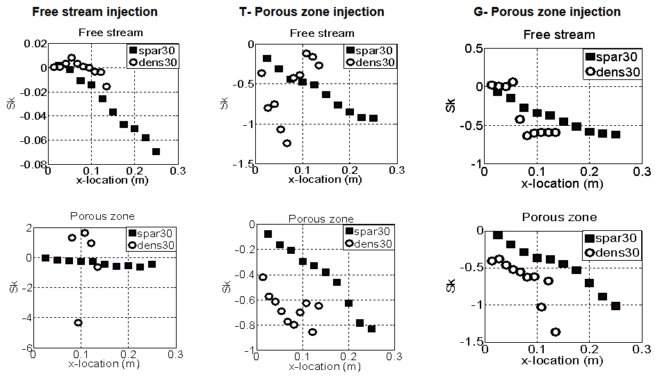 | Figure 6. The skeweness coefficient for both spar30, and dens30 cases results from continuous surface injection scenario. The upper three are for the tracer distribution at the free stream, and the lower are for the tracer distribution at the porous zone |
The results at Figure 7 show that all data is skewed to the right (positive skewness) which means that tracer is moving with the flow. However, the decay of Sk is higher at the porous zone compared to the free stream, which is due to the lower bed porosity which delays tracer movement. Further, it is noticed increase of Sk coefficient values at the porous zone for the two porous zone injection scenarios at location far from the source zone, which is may due to the return of some penetrated tracer back from the free stream. Overall, the difference between pulse and continuous results is that at pulse the injection time is 0.1 seconds with a certain tracer amount is tracked. The variance in continuous injection is maximum close to the source, as tracer is always supported there.
4.2. Tracer Distribution with Distance
The spatial variance was computed for the both pulse and continuous injections to the three injection scenarios. The results were plotted at Figures 7, and Figure 8. Form the Figures, it can be noticed that the spatial variance is increasing at the zone where tracer penetrate to (not the source zone) which is due to vertical tracer distribution with the flow, and indicate that there is a continuous tracer support from the source zone to the other one. The increase of the variance at the porous zone in dens30 case is due to the return of tracer from the free stream again to the porous zone, this conclusion based on the contours plots of tracer concentration [11]. Overall, the spatial variance profile at all injection scenarios follows the same profile published with [6].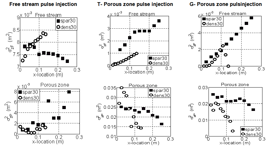 | Figure 7. The spatial variance at all ten different tested locations for both dens30, and spar30 cases. The plots are at the free stream (up), and at the porous zone (down). The injection is at three different locations with pulse injection |
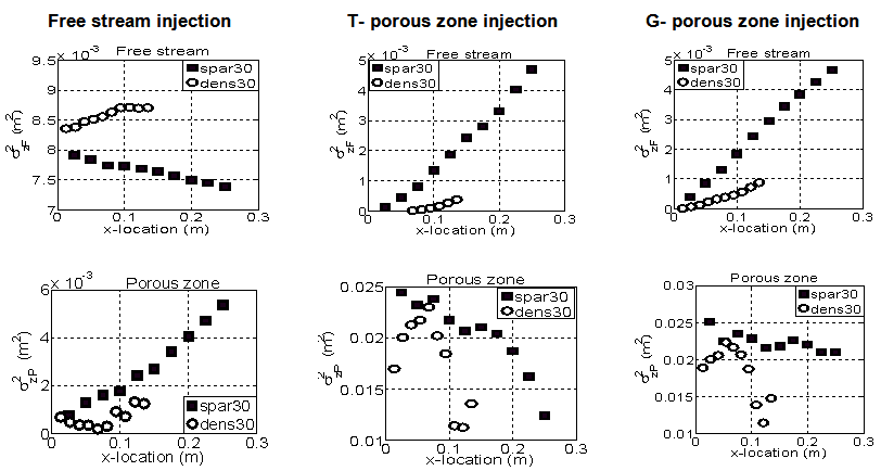 | Figure 8. The spatial variance at ten different tested locations for both dens30, and spar30 cases. The plots are at the free stream (up) and at the porous zone (down). The injection is at three different locations with continuous injection |
5. Conclusions
This paper presents statistical analysis for the tracer dispersion within and over permeable bed. The analysis was for spatial variance, time variance, and skweness. The test is for two different injection scenarios (pulse and continuous). Further, different injection locations were tested for two different porosity mediums. The main concluded points from the analysis are:• The spatial variance profiles tends to decline with the distance from the source zone. However, it increases with the distance for the adjacent zone where the tracer penetrates. That is to say, when the source is in the free stream the variance increases in the porous zone and vice versa. This indicates that the penetration into the adjacent zone enhances mixing within the layer where the tracer was originally injected to, resulting in more homogeneous concentration profile, but not in the adjacent zone.• The pulse injection in the free zone results shows that there is a higher rate exchange between the free stream and porous zone than that when injection is on the opposite situation.• The time variance is higher at the sparse case compared with the dense case.• Overall, the flow heterogeneity causes variety in tracer amount spatially and with time. This makes tracer difficult to be tracked. However, the statistical analysis provided us some sight on tracer migration.
References
| [1] | Paybins, K., Nishikawa, T., Izbicki, J., and Reichard, E., 1998, Statistical analysis and mathematical modeling of a tracer test on the Santa Clara river, Ventura County, California, Water-Resources Investigations Report 97-4275. |
| [2] | Thomson, D., A stochastic model for the motion of particle pairs in isotropic high-Reynolds-number turbulence, and its application to the problem of concentration variance, Journal of Fluid Mech. (1990), vol. 210, pp. 113-153. |
| [3] | Ismail, I., Murali, T., and Mallikarjuna1, P., Statistical Analysis of Groundwater Table Depths in Upper Swarnamukhi River Basin, Journal. Water Resource and Protection, 2010, 2, PP.577-584,doi:10.4236/jwarp.2010.26066. |
| [4] | Smith, R., (2005), An analytical approach to shear dispersion and tracer age, Boundary-Layer Meteorology, vol. 117, January, pp. 383-415; DOI 10.1007/s10546-005-1446-7. |
| [5] | Sukhodolov, A., Nikora, V., Powirski, P., and Czernuszenko, W., (1997), A case study of longitudinal dispersion in small lowland rivers, Water Environment Research, vol. 69, No. 7, pp. 1246 – 1253. |
| [6] | Tanino Y., H. Nepf, (2009), Laboratory investigation of lateral dispersion within dense arrays of randomly distributed cylinders at transitional Reynolds number, Physics Fluids, vol. 21, April, pp. 1-10. |
| [7] | M.V. Prasanna, S. Chidambaram, K. Srinivasamoorthy, Statistical analysis of the hydrogeochemical evolution of groundwater in hard and sedimentary aquifers system of Gadilam river basin, South India, 2010, Journal of King Saud University, 22, PP.133-145, doi:10.1016/j.jksus.2010.04.001 |
| [8] | Elghanduri, N. (2012) "CFD Analysis for Turbulent Flow within and Over a Permeable Bed" American Journal of Fluid Dynamics, vol.2, no.5. |
| [9] | Nordin, C, Troutman, M., (1980), Longitudinal dispersion in rivers: The persistence of skweness in observed data, Water Resource Research ,vol. 16, No. 1, pp 123-128. |
| [10] | Day, T., 1977, Longitudinal dispersion of fluid particles in mountain streams:1. Theory and field evidence, Journal of Hydrology, Vol. 16, No.1, PP. 7-25. |
| [11] | Elghanduri, N. (2015) CFD analysis within and over a permeable bed I: Detail analysis, American Journal of Environmental Engineering, vol. 5, No. 3, 2015. |
 Abstract
 Reference
 Full-Text PDF
 Full-text HTML