1. Introduction

Turbulent mass exchange across the fluid/porous zone is an important task for different engineering aspects, such as: chemical engineering, petroleum engineering, and environmental engineering. Further, studying dispersion of pollutant in rivers and in a porous media is important for designing outfalls water intake and evaluating risks from accidental release of hazardous contaminants. This area of study has been widely covered over three decades (e.g. [1-11]). However, mass exchange across the fluid/porous interface is not fully covered. There are only few laboratory investigations. Yet they are not very detailed. Up to the author's knowledge, the only exception is a series of laboratory investigations of mass transport in flow above and between arrays of vertical cylinders done by Prof. Heidi Nepf’s group. They have provided detailed microscopic information on flow and mass transport quantities. In contrast with the laboratory work, the number of field investigations is huge. However, the field conditions are complex and cannot be controlled. Thus, these data are very difficult to interpret. In addition to the lake of understanding about the mechanisms of mass exchange over flat surfaces. both field and laboratory investigations focused mainly on the effect of bed geometry on the surface/subsurface mass exchange. Overall, it is still a big challenge for scientist and environmental engineers to investigate the tracer dispersion in open channels in detail. The CFD analysis can help to investigate several flow variables in detail. The data estimated can be analysed to improve our understanding about the flow regimes and tracer dispersion in turbulent flow within and over permeable beds.

When the tracer spreads in flowing water, it may take pulse (plump) shape close to the source. Far from the source, it covers the whole flow zone as it is dispersed longitudinally and laterally with the flow. The tracer tracing from that zone is called a surface dispersion. It is named as such because it covers the whole flow zone (vertical surface). Two dimensional (2D) numerical investigations for tracer dispersion within and over a porous zone close to the source (pulse injection) were numerically analysed in detail by [12] The study is a continuation for the previous analysed with the same studied cases. However, the difference between the previous studies and this study is the testing location is far from the source location and the tracer covers the whole flow zone (surface injection).

The main aim of this study is to improve the knowledge of mass exchange across the fluid/porous interface by running a series of CFD simulations. The simulations involve two-dimensional (2D) fully developed turbulent flow within and over an idealized geometry of the porous layer. It is a detailed numerical simulation.

2. The Studied Cases

The studied cases are long flumes with two flow zones; Porous Zone and Free Stream Zone. The Porous Zone consists of rows of rods mounted horizontally at specified distances. The flow zone over the porous zone is called free stream. The studied cases are two, with different bed porosities. The first case is called sparse case (spar30) with a sufficient space between the obstacle for turbulent vortices to form a complete eddies and flow returns laterally. The second case is the dense case (dens30). It is characterized by having small gaps between the obstacles. This causes distinct recirculation vortices at the downstream side of each obstacle and with very shallow penetration of turbulence, which does not go beyond these vortices ([13]). Gambit software was used to build the geometry and mesh for both cases. The simulation was for fully developed turbulent flow within and over permeable bed. Large flumes were built to reach turbulent fully developed regions. Both cases were meshed with coarse mesh to improve the computational accuracy. Figure 1 shows schematic diagram for the columns and rows of the arranged rods bundle symbols for geometry and hydrodynamic characteristics of the simulated cases. The numerical simulation used Fluent within Ansys 12 software. The computing model used is κ-ε turbulent model which is widely used in literature for turbulent flow in CFD simulations. The tracer tracked numerically with the flow using Discrete Phase Model (DPM). The DPM predicts the effect of turbulence on tracer dispersion numerically or analytically. The turbulent model used in this study is the numerical and the tracer tracked using Random Walk Model.

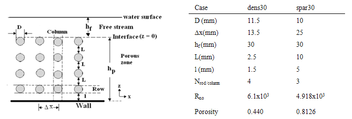Figure 1. Columns and rows of the arranged rods bundle symbols for geometry and hydrodynamic characteristics of the simulated cases

The flowing fluid used is water. The simulation was run as steady state with time until fully developed turbulent flow is reached. The turbulent model used in this simulation was k-epsilon model which is widely used in literature for CFD analysis. This simulation consumed quite a long time to achieve the fully developed turbulent flow in both free and porous zones. This happens due to the large length and the coarse mesh size used. The estimated results were verified with previously published experimental results in [9], and with that published in [14] at the fully developed turbulent zones. A close outcome was achieved for comparing the normalized turbulent kinetic energy (TKE⁺) with normalized bed height for a mid-line between two column rods. Moreover, the normalized velocities (U⁺) versus normalized bed height were verified with previously published work ([12], and [13]).

The tracer experiments were held at the fully developed region in both free stream and porous zones. Discrete Phase Model (DPM) was used for tracer tracking. All tested cases, the tracer injection was over the whole vertical depth to the flow for initially tracer free zone (at t=0, no tracer exist) and tracked over testing time. The resulted data were exported for different time intervals as ascii files. A computer program was built using Matlab Software. This program reads the ascii files. Then it grid the data and scatter it over the whole flow zone. The data then averaged to overcome the flow heterogeneity due to turbulence and upscale the microscopic quantities. Averaging technique is well known technique and widely used to overcome the instantaneous values for turbulent flow variables. In this study, the data was averaged twice (double averaging). The first averaging was from centre to centre between two columns (vertically), then averaging over the flow height.

3. Injection Scenarios

As mentioned previously, the tracer tracked using Discrete phase model (DPM). The DPM is a numerical model included in Fluent Software for tracer injection and tracking in lagrangian frame of reference. In general, the DPM can be used if the mass flow rate is less than 10% of the total mass flow rate (Manual Ansys, 2009). A series of surface injection tracer tests have been carried out. Surface injection tests were run with tracer source covering the whole depth of either the free stream (FS) or the porous zone (T & G). The source locations are shown in Figure 2.

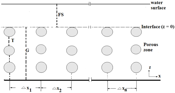Figure 2. Locations of the surface injection in the free stream (FS), and in the porous zone (T, and G)

The simulation was done for both cases using Fluent Software in Ansys 12 as mentioned previously. All simulations start at time t = 0. Then, the tracer is injected into the pollutant-free system so the initial tracer concentration is zero. The tracer injection velocity is always equal to the average velocity at the source. To avoid buoyancy effect the tracer density is set the same as the water density. The total simulation time is 3 seconds, with computing time interval of 0.01 seconds. Regarding the duration of the injection there is a short test called “pulse injection” (duration 0.1s). The raw simulation results consist of a time-series of concentration fields, where each field is defined by a series of values for concentration across the simulation domain at a given time, i.e. by C(x, z, t). The position of the source is varied between the tests in order to cover all the relevant flow regions.

3.1. Pulse Injection

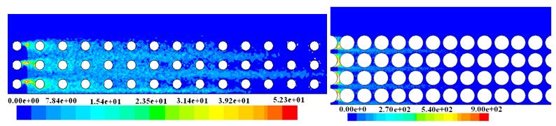
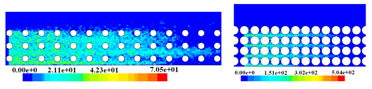
In pulse injection simulations, the duration of the pulse is 0.1 s. The total mass of the tracer injected during this time is 0.07 Kg. The contours of the tracer concentration at different time instances for the three injection scenarios are: Free Surface (FS), Porous Zone at pore throat (T), and Porous Zone in the gap between the rods (G), are shown in Figures 3, 4 respectively.

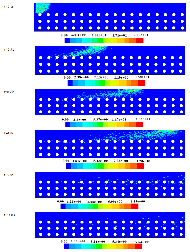Figure 3. Contours of concentration for pulse injection from the free surface zone (FS in Figure 3) at different tested times for spar30 case

Concerning the free stream injection (Figure 2); the movement of the tracer is the quickest close to the free stream surface, and the longitudinal spreading is most pronounced. It is noticed that some tracers enter the porous zone by the time of 0.5 seconds.

Concerning injection in the Porous Zone (Figures 3 and 4). The tracer is the quickest in the injection at the middle gap between the rod-rows (G), where the flow velocity is the highest. This initially forms a ‘wavy’ shape of the tracer plume. Later on, the lateral mixing creates more uniform spread of the tracer. Some tracer moves to the free stream zone. It is then carried forwards by the faster moving free surface flow. It may re-enters the porous zone ahead of the main tracer plume (see for instance t = 2 s in Figure 4).

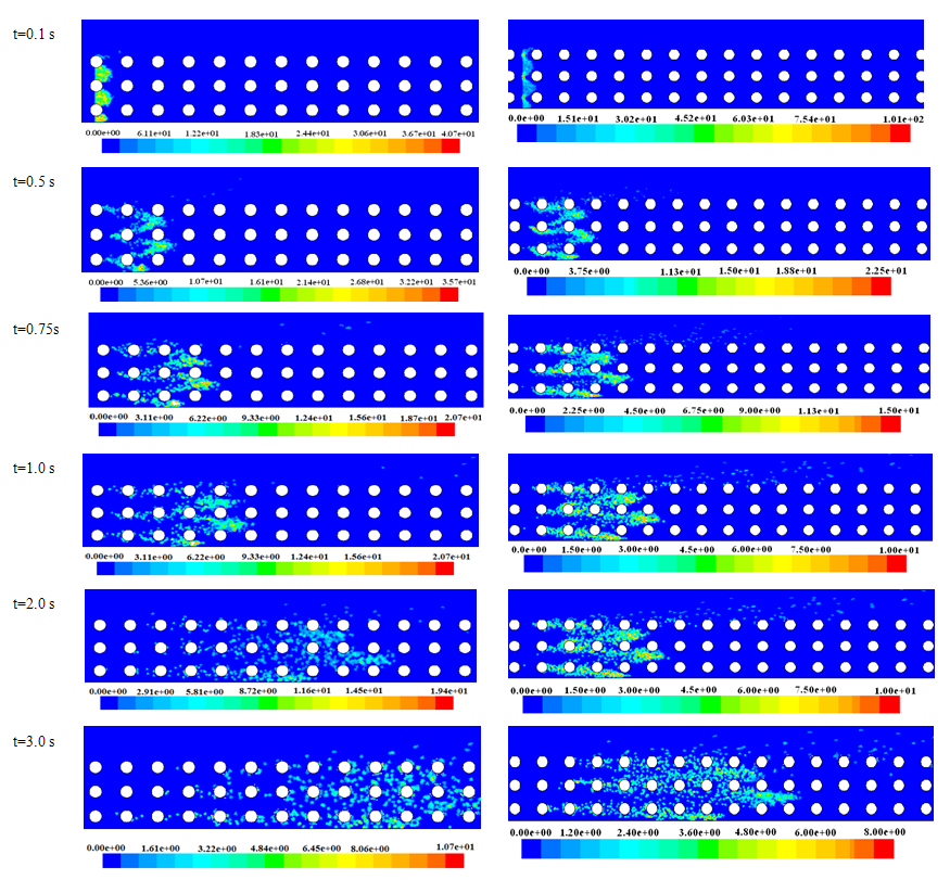Figure 4. Contours of concentration for injection from the porous zone T surface in the left and G surface injection at the right at different tested times for spar30

3.1.1. Free Stream Injection

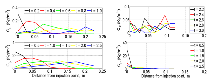
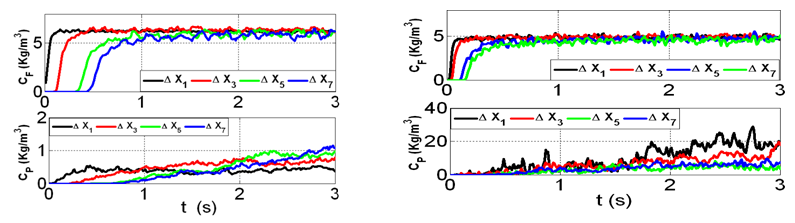
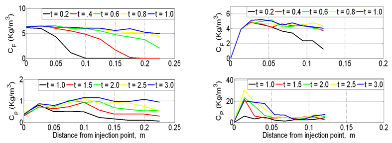
Figures 5 and 6 both show the break-through curves for various x-locations, and the concentration profiles for various time instances respectively. Within the porous zone, the tracer in the dense case took a longer time to appear. It has slower movement with the flow when compared to the sparse case. On the other hand, within the free stream, the break-through curves have similar pattern for both cases.

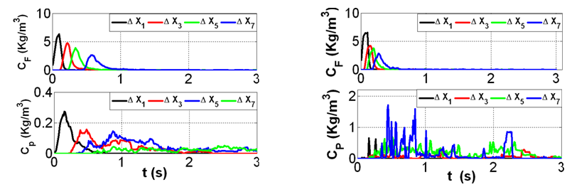Figure 5. Break-through curves in both free stream (top), and porous zones(bottom) for free stream pulse injection for spar30(left), and dens30(right)

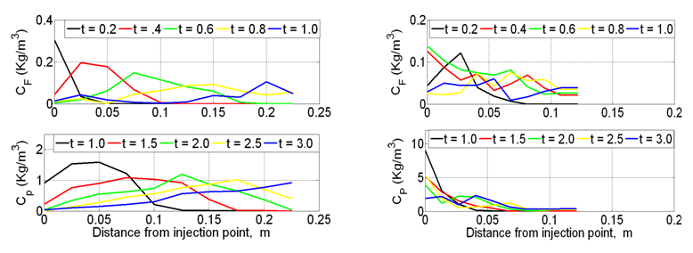
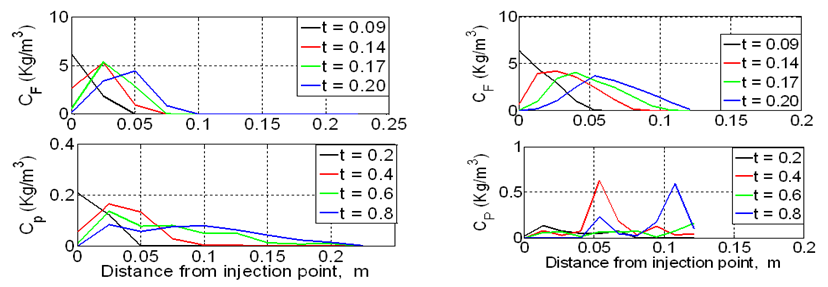Figure 6. Concentration profiles at different times in both free stream (top) and porous zones (bottom) for free stream pulse injection for spar30 (left), and dens30(right)

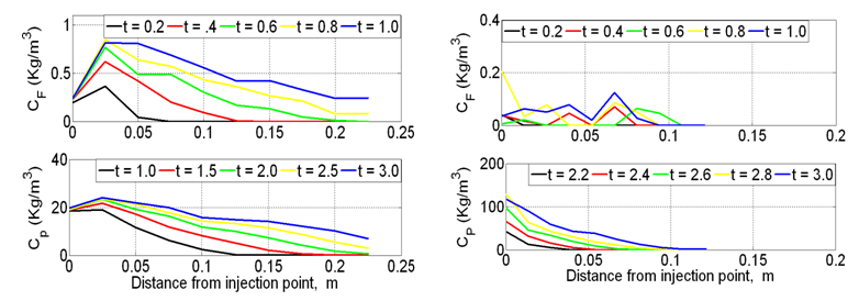
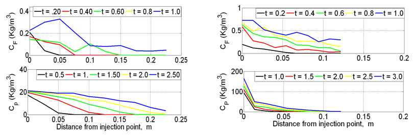
3.1.2. Porous Zone Injection

The breakthrough curves for both free stream and porous zone for the T and G injection surfaces (Figure 2) are shown in Figure 7. It shows that there is a clear distinction between the dense and the sparse cases. Due to much more pronounced mass transfer across the interface; the Spars case has very similar break-through curves for the Porous Zone and the Free Stream zone. They both show the shape typical for dispersion in both open channel flows and the porous media flows. The curves are similar for T and G with the latter one having somewhat more pronounced mass exchange when compared to the point sources of injection, these curves have a pronounced tail i.e. they are more asymmetric.

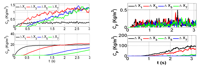
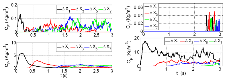Figure 7. Breakthrough curves in both free stream (top), and porous zones (bottom) for porous zone surface pulse injection (T) for spar30 (left), and dens30 (right)

The exchange across the interface for the dense case is more intermittent especially for the T surface. Following the injection from the surface, tracer is found in the free stream only for a short period of time, and with small concentrations. For G surface, the residence time in the Free Stream is longer and the concentration levels higher, but still very small compared to those in the subsurface.

Figures 10 and 11 show the concentration profiles after T, and G injection. They confirm the distinct between spars, and dense case described above.

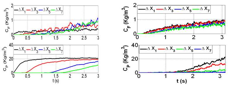
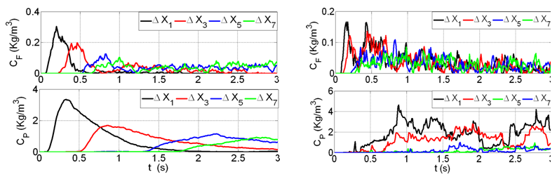Figure 8. Breakthrough curves in both free stream (top), and porous zones (bottom) for porous zone surface pulse injection (G) for spar30 (left), and dens30 (right)

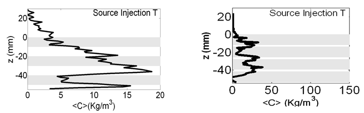
Figure 9. Concentration profiles in both free stream (top) and porous zones (bottom) for total porous zone surface pulse injection (T) for spar30 (left), and dens30 (right), t is the time in seconds

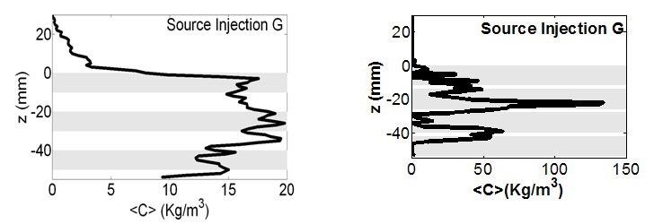
Figure 10. Concentration profiles in both free stream (top) and porous zones (bottom) for total porous zone surface pulse injection (G) for spar30 (left), and dens30 (right) cases), t is the time in seconds

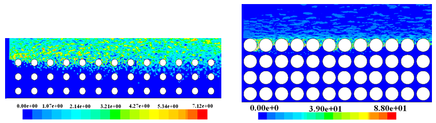Figure 11. Contours of tracer concentration (Kg/m3) after 3.0 (s) of injection from a surface source covering the whole free stream depth (FS) in Figure 2 for spar30 (left), and dens30 (right)

3.2. Continuous Surface Injection

The tracer is injected at the same surfaces as in pulse surface injection. The mass injection rate for all scenarios was constant and equal to 0.0278Kg/s.

3.2.1. Free Surface Injection

Figure 12 shows an example of the contours of the tracer concentration for free surface injection. The penetration of the tracer into the subsurface can be observed in Figure 12. As the observation point moves downstream the tracer penetrates deeper. However, the penetration to the porous zone is higher in the dense case. This is due to the flow pattern in the interface which is discussed in detail by [13].

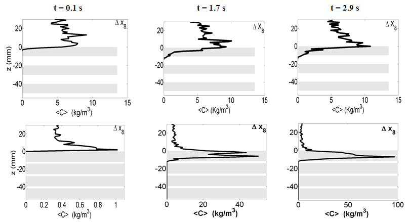Figure 12. Vertical concentration profiles for spar30 (Top), and dens30 (Bottom) for continuous free stream surface injection at different time levels (grey colour represents the rods location)

Quantitative distribution about the tracer penetration into the porous layer can be observed at the vertical concentration profiles shown in Figure 13. The profiles are plotted for three different time intervals. From the Figures, it can be noticed that the distribution is irregular with the largest concentration values within the interface zone. This pattern of concentration agrees with Ghisalberti, and Nepf (2005), and Okamoto, and Nezu (2010), where the tracer amount also builds up within the interface zone. A larger tracer amount accumulates within the interface with smaller mass penetration thickness in dens30 case compared to the spars one. It was at dens30 nearly double that at spar30. Furthermore, the plots of dens30 case show that the maximum tracer concentration is within the porous zone, and not over the top rod (z = 0) as that shown at the spar30 case.

Figure 13. Breakthrough curves in both free stream (top), and porous zones (bottom) for continuous injection from a surface source covering the whole free stream depth for spar30 (left), and dens30 (right)

Figure 14, shows the break-through curves for various locations. From this figure, it can be noticed that, the tracer concentration in the dense 30 case reaches steady state in shorter time compared to the sparse case. This is due to the larger flow velocity. Moreover, it shows a better contact between the free stream and porous zone in spar30 case when compared to the dense case. On the other hand, within the porous zone, at the dense case, the tracer took longer time to enter the first tested zone. Then it built up to a large concentration values with time as it is trapped in between the rods. At the spars30 case, tracer passes within the porous zone smoothly with time to reach steady state at each tested zone. However, far from the injection source, the tracer movement is smooth. This is might happened as a result of the tracer that moving with the main flow between two rows and do not expand at the zone between the rod columns.

Figure 14. Stream wise averaged concentration in both free stream (top) and porous zones (bottom) for total continuous free stream for spar30 (left), and dens30 (right)

Figure 15 shows steady state concentration change within the free stream at different tested locations. This Figure shows that within the porous zone, the tracer in sparse case moves smoothly with the flow. However, most of the tracer at the dens30 case get trapped close to the source zone, and small amount of it moves to a further distances.

Figure 15. Contours of tracer concentration after 3 (s) of injection from the surface source covering whole porous zone (G) (Figure 2) for spar30 (left), and dens30 (right)

3.2.2. Porous Zone Injection

Figure 16 shows the contours of tracer concentration after 3 seconds of porous zone surface injection. The tracer moves faster in the middle i.e. between rod-row 2, and 3 smoothly within sparse case compared to dens30. Interestingly, close to the source, the tracer moves backwards, i.e. against flow direction and its concentration is the highest value. This is due to the stationary vortices behind the rods, which trap a significant amount of tracer and move it in a circle. Furthermore, around the last upper rod (first rod on the right side), some tracer moved from the free stream back into the porous zone.

Figure 16. Contours of tracer concentration after 3 (s) of injection from the surface source covering the whole porous zone (T) (Figure 2) for spar30 (left), and dens30 (right)

The vertical tracer concentration change with bed height was examined for both T, and G injection scenarios. The simulation time was increased from 3 to 5 seconds to ensure that steady state is reached. Figure 17 and Figure 18 show the resulting vertical concentration profiles. Spar30 case results show a better tracer mixing within the porous zone and across the interface. The tracer mass transfer across the interface is much stronger for G injection for both cases. Within the porous zone, the tracer at the dense case moves in channels within the rows with higher concentrations at the lower part of the porous zone.

Figure 17. Vertical concentration profiles for both spar30 (left), and dens30 (right) case for T surface injection after 4.9 s injection for ∆x=2 (grey colour represents the rods location)

Figure 18. Vertical concentration profiles for both spar30 (left), and dens30 (right) cases for G surface injection after 4.9 s for ∆x=2 (grey colour represents the rods location)

The break-through curves for the two different surface injection scenarios are shown in Figures 19, and 20 respectively. The plots for surface injection (G) in spar30 show a good contact between both free stream zone and the porous zone. Within the porous zone, the tracer movement was nearly stagnant at the more dense case. It is also built up at each zone to reach high concentration levels. The tracer at the porous zone reached steady state at the spars case within the tested region. However, in dens30, it continued to build up within the testing time. On the other hand, the surface injection (T), shows the same overall pattern, but with some differences. It also shows a better contact between free stream injection and porous zone for the dense Case.

Figure 19. Breakthrough curves in both free stream (top), and porous zones(bottom) for total porous zone continuous injection(G); spar30 (left), and dens30 (right)

Figure 20. Breakthrough curves in both free stream (top), and porous zones (bottom) continuous injection (T); spar30 (left), and dens30 (right)

The stream wise spread of tracer through longitudinal distance for both porous injection cases T, and G are shown in Figures 21, and 22 respectively. Both figures show that the tracer amount in the porous zone reaches the largest value close to the source of injection and decreases gradually. This indicates that tracer moves slower in the porous zone. For the dens30 case, tracer could not enter some tested zones far from injection surface because of the low velocity within the porous zone.

Figure 21. Stream wise averaged concentration in both free stream (top) and porous zones (bottom) for total porous zone continuous injection (G); spar30 (left), and dens30 (right), t is the time in seconds

Figure 22. Stream wise averaged concentration in both free stream (top) and porous zones (bottom) for total porous zone continuous injection(T); spar30 (left), and dens30 (right), t is the time in seconds

Overall, the tracer concentration within the porous zone is higher than that at the free stream. This may indicate that the tracer movement from the upper zone to the lower zone is the larger than that in the opposite direction or that the higher flow velocity in the free stream moves the tracer faster. Furthermore, at the porous zone, it is noticed that an amount of tracer returns against the flow direction in surface injection (T). This is due to the presence of vortices between the two obstacles. Overall, the vertical velocity has a larger effect on the tracer velocity within the porous medium.

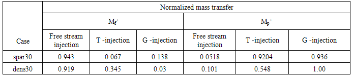
4. Mass Distribution between Free Stream and Porous Zones

The normalized mass flux, M⁺, through the centreline between two rod-columns was calculated as mass flux of tracer at any time divided by the mass input at the source (), where the tracer mass flow rate was computed as () at each zone. The normalized mass transfer was plotted versus the normalized time at the tested zone ( ) for the three injection scenarios for both spar30, and dens30.

Table 1 shows that at the steady state even though the tracer distributes with larger amounts at the source zone, there is reasonable amount of penetration to the other zone. For the free stream injection, tracer at the denser case penetrates with larger percentage to the porous zone compared with the other case. On the other hand, the two porous injection zones show different results. The larger the bed porosity, the better the contact between the tested zones will be. Figure 23 shows the difference in mass penetration between the free stream and the porous zone for both spar30, and dens30 cases. Both Table 1 and Figure 23 show that the steady state can be reached faster in the free stream injection when compared to porous zone injection. Further, T injection scenario shows better tracer penetration from the source zone to the other flow zone.

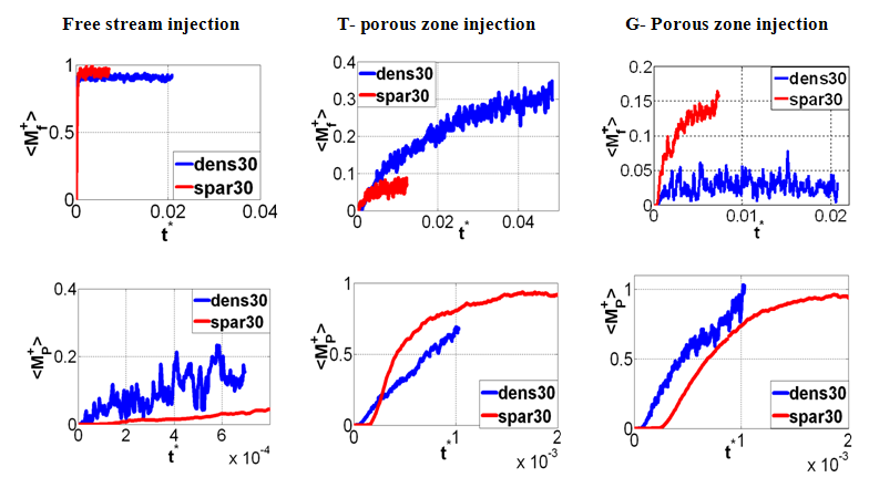Figure 23. The mass of tracer at both free stream (top), and porous zones (bottom), for both tested cases. The results are at (∆x=2) for the three injection scenarios

Table 1. Normalized averaged mass transfer at both free stream and porous zone for the three-tested case, for both spar30, and dens30 cases at (∆x = 2)

5. Conclusions

This paper provided an insight into the tracer dispersion in fully developed turbulent flow over and through a permeable layer. Two different cases are compared: (i) The Sparse Case with a sufficient space between the obstacles for turbulence from the free surface zone to penetrate deep into the porous zone, (ii) Dense Case with very small gap between the obstacles. It is characterised by distinct recirculation vortices at the downstream side of each obstacle with very shallow penetration of turbulence.

Two different injection scenarios and three different tracer feed sources were simulated: a rapid release of a limited mass of tracer, called pulse injection and a continuous release at constant rate, called continuous injection. For each scenario, a series of locations of surface tracer source have been tested. The contour plots of the tracer concentration are presented in order to provide visual information of the tracer pathways. Both spatially averaged results in the form of concentration profiles at various time instances and breakthrough curves for various locations, both of them provide more concise information, which allows a quantitative analysis. The analysis includes the influence of porosity of the permeable layer on the tracer migration and fluid/porous exchange.

The main conclusion points from the analysis are:

• The results of the pulse injection within the free stream show that the exchange with the Porous Zone occurs faster for the Sparse Case than for the Dense Case.

• During the surface injection within the Porous Zone, the location of the injection surface has some effect on the tracer migration. The injection surface in the middle of the vertical gap between the obstacles (G-injection) resulted in faster penetration into the free stream than the injection across the narrow throats of the horizontal pores (T-injection).

The vertical profiles of the tracer concentration across the free surface zone thickness show a considerable difference between the sparse case and the dense case. In the former case, the tracer is spreading across the whole free stream and over the top row of cylinders. However, in the latter case practically all of the tracer has been trapped within the top row of cylinders. The maximum concentration for the spar30 case occurs at the interface and gradually declining at the observation point whether it moves into the free stream zone or into the porous zone. On the other hand, the concentration profile for the Dense case the concentration profile practically exists only over the top row of cylinders and shows a sharp decline at their upper and lower edge. This is a result of the stationary recirculation vortices which trap all of injected trace.

Nomenclature

A = cross sectional area, m²

C₀ = Solute concentration at the source, Kg/m³

C_F = Averaged, spatially averaged solute concentration in the free stream, Kg/m³

= Free stream spatially averaged concentration, Kg/m³

Cp = Porous bed averaged, spatially averaged solute concentration, Kg/m³

= Porous zone spatially averaged concentration, Kg/m³

D = Rod diameter, m

m = the total solute mass, Kg/s

m₀ = the inlet mass of tracer, Kg/s

M_F⁺ = Normalized mass at the free stream

M_P⁺ = normalized mass at the porous zone.

t = Time. s

t* = Dimensionless residence time.

U = the average velocity, m/s

x = Longitudinal coordinate, m

z = Vertical coordinate, m.