Carl Y. H. Jiang
Faculty of Science, Engineering and Built Environment, Deakin University, Victoria, Australia
Correspondence to: Carl Y. H. Jiang , Faculty of Science, Engineering and Built Environment, Deakin University, Victoria, Australia.
| Email: |  |
Copyright © 2014 Scientific & Academic Publishing. All Rights Reserved.
Abstract
A novel method of bottom-up bathymetric modelling in investigating the quality and quantity of seriously polluted water in large scale inland lake has been proposed. This method is fully integrating remote sensing imagery with digital elevation model and spectral reflectance data. Setting the water bottom up is a mathematical treatment to overcome the most difficulty originated from the complexity of water bottom shape, and then depths of water are measured directly. The proposed method does not rely on the spectral reflectance and digital number like other methods to perform bathymetric modelling. In this approach, another method used in bathymetric modelling has also been proposed. In order to get a comparison with other research manners, the spectral reflectance data supplied by MODIS have been used in both investigating the quality of polluted water and reverse test. However, the detected depths of water in inland lake based on spectral reflectance are not reliable. The area of water surface and perimeter of boundary between water and land were easily calculated by the knowledge of digital image processing. Of importance is that the water locating at high level geographical positions but captured by satellite from sky and stored in remote sensing imagery as one part of water body in lake have been trimmed off before the detected data of lake were further used because this parts of water result in fatal errors. The volume of water body was calculated by computational geometry, the potential vital error generated by improperly selecting water body has been demonstrated in the process of calculation. Some concerned topics relevant to the data of water body depths hidden in digital elevation model have also been included and discussed briefly.
Keywords:
Bathymetric modelling, Remote sensing imagery, Digital elevation model, Spectral reflectance, Inland lake, Polluted water, Water storage
Cite this paper: Carl Y. H. Jiang , Bottom-up Bathymetric Modeling in Investigating Quality and Quantity of Highly Polluted Water in Large Scale Inland Lake Using Remote Sensing Imagery and Digital Elevation Model, American Journal of Environmental Engineering, Vol. 4 No. 5, 2014, pp. 117-141. doi: 10.5923/j.ajee.20140405.05.
1. Introduction
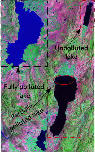
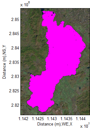
Bathymetric modelling ReviewBathymetric modelling is a very popular research topic, thousands reports have been published. However, the most of researches by means of different approaches have a similar problem, hence the most of researchers fail to tell what exact absolute depths of water and only indicated relative variation of interested parameters related to water in lakes or rivers [1-6] in the process of using remote sensing imageries. They were able to passively use the information supplied by remote sensing imageries. But they may not realize a fact that the data supplied by satellites for users fail to uncover some intrinsic factors of observed objects on the earth, which plays a dominant role in determining the physical or physiochemical properties of substances.Some researchers try to resolve the complexity of water bottom by means of statistical model [7], as a matter of fact, this approach is impossible to reach to the reality as nobody can model the terrain on the earth surface using any mathematical models. The bottom albedo-independent bathymetry [8] is a popular algorithm used in bathymetric modelling, however it fails to verify water positioning at high levels but captured by satellite as one part of water body. That could lead to fatal errors without three-dimensional examination. Unfortunately, thousands researchers in the world including commercial package developers have been applying this algorithm into different research fields.Such fatal error is very difficult to be found by researchers in the world if they fully rely on the remote sensing imageries. This potential fatal error is to be indicated by author in this paper.About Bathymetric Modelling of Fully Polluted Inland Lake The fully polluted inland lake to be studied is located at the following geographical location.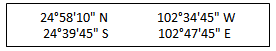 The lake is called as Dian Chi which locates in Southwest China having over 1800 meters elevation. It has been polluted for over three decades (see Figure 1 and Figure 2). It looks very dirty, the local government has been seeking for a best resolution to treating it. Except for pollution, this lake is very large and looks like an inland sea, the shape of water bottom is very complex, and it is difficulty to have reliable hydraulic data of it. Therefore, several trials to treat it have failed. In other words, traditional manners fail to detect the depths of water and obtain other hydraulic parameters in this lake accurately. It must find out a new and effective manner to detect and measure this large scale inland lake.
 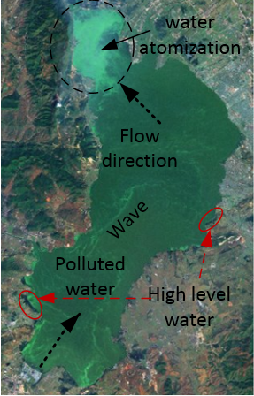 | Figure 1. Over view of highly polluted lake (Landsat 7) |
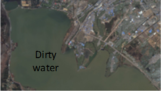 | Figure 2. Partial view of highly polluted lake (Landsat 8) |
Objectives of researchOn the basis of specific requirement for treating this lake, a new method of detecting depths of water body and calculating its surface area, volume and perimeter is to be proposed. The brief contents of the research to be performed are shown as follows.1. Select a clear remote sensing imagery and corresponding digital elevation model (DEM).2. Select the spectral reflectance having the same date or period as the one when the remote sensing imagery was captured.3. The same dimension of remote sensing imagery, DEM and the spectral reflectance data are required. 4. The detected lake in the digital image must be verified by using three-dimensional DEM, and then trim some edges and spots which do not belong to the lake off before the data related to the detected lake can be further used.5. The absolute depths of water body are obtained by using bottom-up new technique. Another manner is also to be discussed.6. The spectral reflectance data selected from NASA MODIS must be accurately melt into the corresponding lake surface area. In this research, the data with properties of black-sky, band 3(blue), Nadir and local solar noon are selected to investigate the quality of water in the lake. 7. Calculating the volume of water body is based on computational geometry.8. The surface area and length of boundary between water body and land are calculated by using the technique in the conversion between colour digital image and black-white image.Meanwhile, in order for readers to conveniently access to the research target, some basic theory is to be reviewed and the new concepts proposed by author is to be introduced and explained in detail. Eventually, in order for ones to instantly understand some secrets hidden in DEM about lakes or rivers, additional concerned topics are to be further discussed briefly and provide ones with potential applications in the last section of conclusions after the outcome of modelling being generated.
2. Methodology
In the following subsections, several relevant concepts originated from multidiscipline are to be briefly reviewed and the techniques created for this research are introduced as well so that one can access to the core of problems quickly.
2.1. Inherent Optical Properties of Water
Classification of Optic properties of WaterIn order to easily distinguish properties of water in different research fields, the optical properties of water are already divided into two mutually exclusive classes: inherent and apparent [1]. Such classification may be able to be identified by terms: extinction coefficient and attenuation coefficient. At laboratory level with same operational conditions, two terms may not have much difference, however researchers are accustomed to use the term of attenuation coefficient to describe how the solar intensity decays when it penetrates through such as atmospheric layer or into water in lake. The attenuation coefficient usually is the sum of adsorption coefficient and scattering coefficient in terms of the form of solar radiation loss in media. The detail is shown in the following subsections.Geometric Feature of Energy Source Penetrating into WaterThe inherent optic properties of water can be explained by assuming a continuous beam with incident energy (in the form of power, thus spectral power) EI(λ) (W∙μm-1) penetrating into a cubic volume ΔV (m3) of water at wavelength λ or wavelength interval (see Figure 3), in which ΔL(m) is thickness of water, ∆A (m2) is surface area (rad) is scattering angle with 0≤ψ≤π and ω (sr) is a solid angle. The incident light travelling within water can be portioned into three parts in terms of energy: transmitted energy ET(λ), absorbed energy EA(λ) and scattered energy ES(λ). In this case, all of them are regarded as a function of wavelength λ (μm) respectively.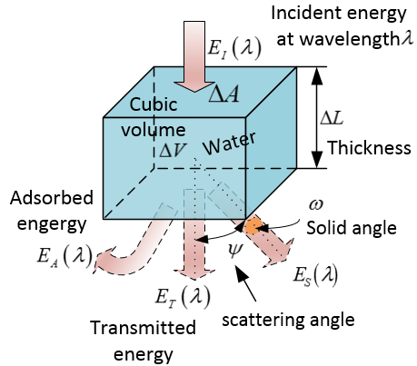 | Figure 3. Schematic of spectral power penetrating into a unit volume of water |
They are then expressed by the following dimensionless coefficients respectively.Spectral absorptance A(λ):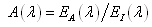 | (1) |
Spectral transmittance T(λ):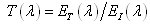 | (2) |
Spectral scatterance S(λ):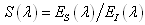 | (3) |
It is easily found that 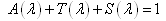 | (4) |
The further approach for above coefficients is that on the basis of Figure 3 and concerns (the spectral “colour” of water caused by scattering), the coefficients can be shown by the following types when the geometric size of water volume approaches to zero so that the hydrologic optics can be achieved.Spectral absorption coefficient (λ):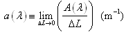 | (5) |
Spectral scattering coefficient t(λ):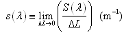 | (6) |
Spectral beam attenuation coefficient (λ) is then defined as 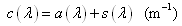 | (7) |
Following up above definitions, another useful concept in interpreting scattering phenomenon is spectral volume scattering function (ψ; λ), which is defined by the fraction of incident spectral power distributing along scattering angle ψ per unit distance ΔL and unit solid angle Δω.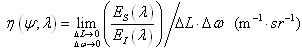 | (8) |
Spectrum of Solar Radiation Incident into Water The spectrum of the solar radiation reaching lakes surface and the effect of different wavelengths on organic matter and living organisms is shown by Figure 4. The radiation in the visible range 400-700 nm and is usually called Photosyn thetically Active Radiation (PAR). Figure 4 is useful in the process of investigating lakes.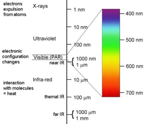 | Figure 4. Spectrum of solar radiation [9] |
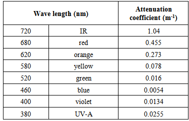
Of importance is that the attenuation of solar radiation in media varies with wavelengths. The attenuation coefficient for pure water is supplied in Table 1. Based on those data, it is useful to assess how the water in lakes is polluted when one band light is selected to investigate the quality of water in lakes containing such as living phytoplankton or pollutants and so on.Table 1. Attenuation coefficients of wavelengths in pure water [9]
 |
| |
|
Depth of Monochromatic light Penetration Another important issue is about how much depth individual light is able to penetrate into water. The information of monochromatic light penetrating into the pure water is supplied in Figure 5. As seen, the depth of the blue light penetrating into water is more than the one which others can do. In fact, at blue wavelengths, photons are barely energetic enough to boost electrons into higher energy levels of the water molecule, and the photons do not have the right energy to interact easily with the molecule as a whole. Only some vibrational modes of the molecule can be excited, therefore the photons do not interact strongly with the water molecules [10]. On the basis of this fact, the blue light is chosen to study the polluted water combining with reflectance offered by NASA MODIS in this research.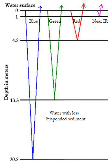 | Figure 5. Depth of monochromatic light penetration [11] |
2.2. Apparent Optical Properties of Water
In the last subsections, some definitions of inherent optics properties of water are already introduced. However, apparent optical properties of water in lake connecting with remote sensing is much complex. In order to simplify the case, the attention is only paid to the mechanism of solar light penetrating into water and how the satellite receives signals from the water surface (see Figure 6). 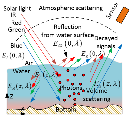 | Figure 6. Schematic of solar light scattering, adsorption and reflection in water body and on water surface |
Decay of Solar RadiationThe decay of solar radiation penetrating into water on the Earth is similar to the case which it travels within atmospheric layer. According to Bouguer’s law (or say Beer–Lamber law), the incident spectral power of beam Eλ is decayed at depth z=L from water surface z=0(see Figure 3 and Figure 6), which can be expressed by 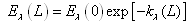 | (9) |
Where, kλ(L) is the optical thickness defined by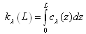 | (10) |
Where, cλ(z) is spectral attenuation coefficient which can be obtained from equation (7), z is a variable in the vertical direction. Because it is difficult to find it, the right hand side of equation (10) is usually replaced by the term (Kλ∙Z,), where Kλ is mean spectral attenuation coefficient and assuming that a medium has uniform composition, pressure and temperature. Thereby, equation(9) is rewritten as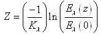 | (11) |
Where Z is the depth of water body. The term Eλ(z)/Eλ(0) is spectral reflectance which is to be replaced by MODIS spectral reflectance [12] to examine the quality of water once the absolute depth of water is known.Colored Water and Decayed Signals Received by SatelliteThe water “colour” and decayed signals received by satellite are different concept and process but they have potential correlation, which can be explained by using the spectral power shown in Figure 3. When the solar light reaches a water surface (z=0), the solar spectral power EI(0, λ) can be further expressed as the following relation: | (12) |
Where• ESR(0, λ) is spectral power which is specularly reflected at the water surface (the mirror effect), which is then received by the sensor of satellite in the form of spectral signal, but they have less valuable information.• ET(z,λ) could be converted into EA(z,λ) and ES(z,λ) when the solar beam travels within water along the path L. • ES(z,λ) is backscattered into the water surface to be ER(0,λ). This part spectral power is also received by the sensor of satellite in the form of spectral signal as well. The more useful information including coloured water is contained. Specular reflection is equal at all wavelengths, but absorption and backscatter produce distinctive spectral signature, thus water is represented as specific “colour”. Very clear, such the “colour” of water is caused by adsorption and scattering rather than reflection at water surface [13]. The absorbed energy is used to heat water. Red and NIR band radiation is easily to be absorbed by water respectively. However, for highly polluted water, more solar energy could be absorbed because of other substances (pollutant) existing in the water, thus the mixed capacity of heat is larger than the one of pure water. The “colour” of water could approach to blue or green depending on the concentration of pollutants in water.
2.3. Bidirectional Reflectance Distribution Function and Albedo
The bidirectional reflectance distribution function (BRDF) is a four-dimensional function to describe how incident solar radiation reflects from surface in a specific solid angle with specific zenith angle and azimuth angle (see Figure 7).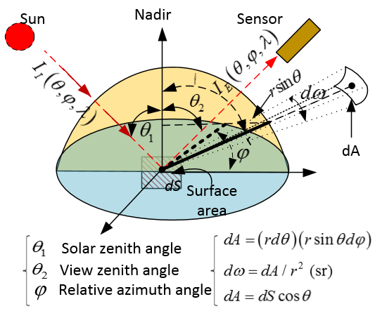 | Figure 7. Schematic of bidirectional reflectance distribution function |
Several definitions are very important in understanding how data are captured and shown by the satellite. They are briefly reviewed as follows [14]. The attention should be paid to individual unit.Solid Angle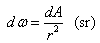 | (13) |
Spectral Intensity (Radiance)The spectral intensity (radiance) is defined as follows.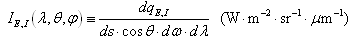 | (14) |
Where, the subscript E,I denotes emit or incident, hence solar powerd q (W) leaves or enters the surface dS per unit solid angle and wavelength interval dλ about λ in direction (θ, φ) through surface dA.Spectral Radiation Flux The emitted or incident spectral radiation flux is defined by equation(15) respectively. 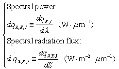 | (15) |
Thus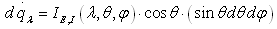 | (16) |
Spectral AlbedoThe spectral albedo αλ is defined as follows in terms of the definition of spectral power. | (17) |
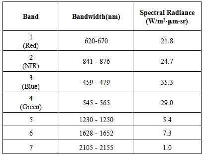
White-Sky and Black-Sky AlbedoWhen solar beam travels within atmospheric layer, it is portioned into direct beam and diffuse beam. The cases of white-sky (only diffused solar beam exists) and black-sky (only direct solar beam exists) albedo are two extremes. The rest albedo is required to calculate by using other parameters such solar zenith angle. NASA MODIS provides several reflectance data which are based on this principle without considering atmospheric correction for different users [12, 15].Table 2. NASA MODIS Bands [16]
 |
| |
|
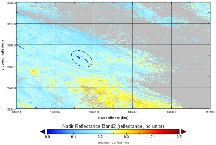
It is easy to select desired spectral reflectance data according to bandwidth and view angle (see Table 2). In this research, the 16-day reflectance data containing Band 3 (blue) and view angle of Nadir at local solar noon are chosen. The figures of selected data are represented in Figure 8−Figure 10. They were made from 01/January/2014. The spectral reflectance data (blue band) containing the selected lake is to be further extracted from Figure 10 for modelling.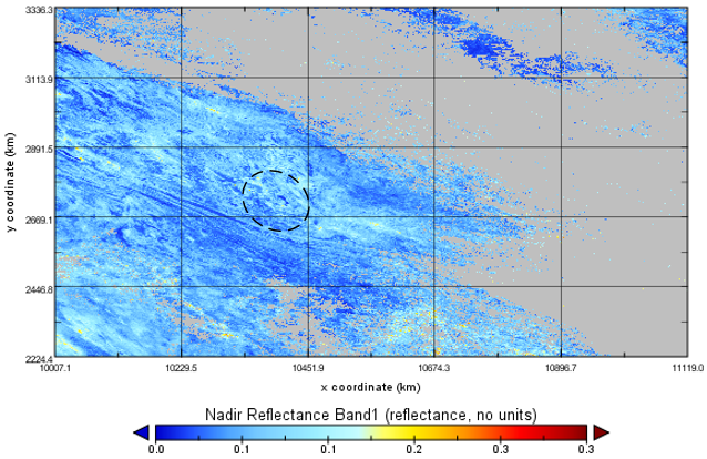 | Figure 8. Selected MODIS nadir reflectance in band 1(Red) |
 | Figure 9. Selected MODIS nadir reflectance in band 2 (NIR) |
 | Figure 10. Selected MODIS nadir reflectance in band 3 (Blue) |
2.4. Spectral Signature of Highly Polluted Waters
Some typical signatures of objects in landscapes are shown in Figure 11. For highly polluted water, it does not have specific signature because the component of water mixture is complex. However, the colour variation of water provides one of useful evidences to prove what a degree the water is polluted.As mentioned before, according to thermodynamics, the heat capacity of one substance mixture is always larger than the one of pure substance. Thus the system (in this case, which is water body) consisting of mixture requires more energy to heat mixture than the one of heating a pure substance to reach to the same temperature. In this case, more solar energy absorbed by water and pollutants in the investigated lake compared with neighbouring unpolluted lake results in the distinctive colour of water shifting to blue colour (see Figure 12). 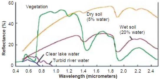 | Figure 11. Spectral Signature of common objects in landscapes [17] |
 | Figure 12. Landsat TM, colorcomposite RGB pan sharpened by band: 7, 4, 2 |
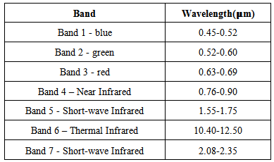
The bands for Landsat TM is offered in Table 3 for easily reading. On the other hand, because of that, the lower reflectance is displayed by Red and NIR band in Figure 8 and Figure 9 respectively. Furthermore, the signal retrieved by blue band does not show significant reflectance from investigated lake (see Figure 10). That could be a typical feature for highly polluted water.Table 3. Landsat TM Bands [18]
 |
| |
|
2.5. Technique of Integrating Remote Sensing Imagery with DEM
In the last subsections, some concepts related to remote sensing are already reviewed. However, the focus on this research is different from others in this field. The technique of integrating remote sensing imagery with DEM created by author are already applied into different applications. In order for one to understand it, its principle is introduced as follows briefly. Both remote sensing imagery and DEM are built on a matrix when they are made on their own platforms. Of importance is to ensure both of them have the same dimension before they work together. The individual information is transferred by linear indexes. The detailed explanation is represented in Figure 13. The data can be accurately transferred and displayed by using this technique. The example of application is to be shown in the following subsections.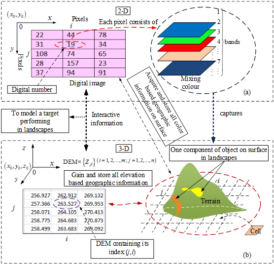 | Figure 13. Principle of integrating remote sensing imagery with DEM |
2.6. Select DEM and Remote Sensing Imagery for Modelling Polluted Lake
As mentioned above, to model depths of water DEM and corresponding remote sensing imagery are required. They are shown in Figure 14 and Figure 15 respectively. The dimension of them is 1146×750. Both of those products are supplied by NASA and USGS (however, they usually provide users with the data of various satellites mutually within those two US departments) respectively. 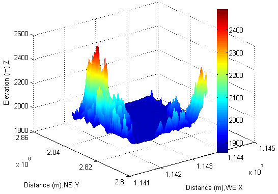 | Figure 14. Selected NASA SRTM3DEM (1146×750) for modeling |
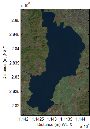 | Figure 15. Selected USGS Landsat 8 Remote Sensing Imagery (1146×750) for modeling |
The date of remote sensing imagery in Figure 15 was captured on 01/January/2014 at local noon time.
2.7. Detect Lake and Display it into DEM
The lake shown in Figure 15 can be quickly detected by specifying a pixel location of lake and corresponding individual value of R (Red) G (Green) B (Blue). The performance is carried out by using MATLAB®.The detected lake is then coloured by red to distinguish it from other objects shown in the imagery (see Figure 16). The most important is that each pixel marked by red colour contains individual linear index behind each pixel. On the other hand, at this stage, each pixel also stores digital number (DN) which can be associated with many issues in remote sensing technology. 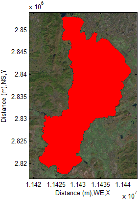 | Figure 16. Detected lake (red) in imagery (1146×750) |
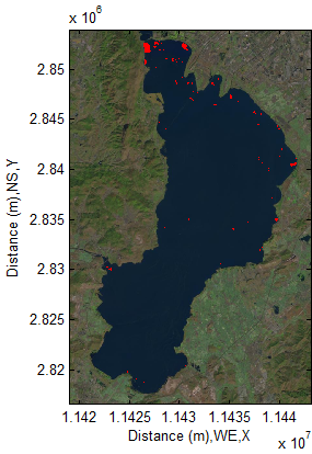
At next step, obtained linear indexes are able to display the elevation of lake in DEM. In order to clearly visualize lake in DEM, the lake is raised by adding 80 meters to original elevation of it before it being transferred into DEM (see Figure 17). Now, the task of transferring the most important information (data) is done. In the next subsection, the technique of linear indexing is used to display corresponding spectral reflectance.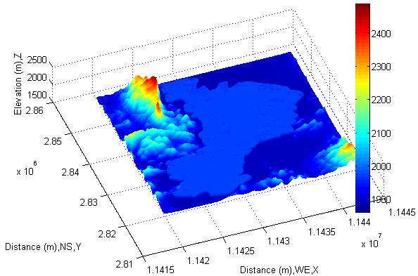 | Figure 17. Display detected lake into DEM (1146×750) |
2.8. Classify Reflectance and Display
As mentioned previously, MODIS offers divers spectral reflectance for users. Although those data were already recontracted by correcting atmospheric factors, they fail to be used into modelling directly. The same thing which can be done is to accurately index those data. Of importance in the process of dealing with reflectance data is distinguishing land and lake firstly by classifying their individual linear indexes. Once classification is successfully done, the corresponding spectral reflectance of lake and land is capable of being displayed (see Figure 18). Its significance is that the spectral reflectance measured by MODIS is then able to helpfully investigate some uncertain facts such as the quality and depths of water.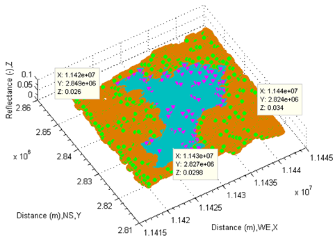 | Figure 18. Show classified reflectance on surface of lake and land |
2.9. Trim Irrelative Edges and Spots off
In the last subsections, although the lake is successfully detected according to the unique feature of water (the chemical elements of water is not affected by pollutants in lake), it cannot guarantee that whole water recorded by remote sensing imagery is located within the lake. To verify it, what can do is that at first display whole elevations of detected objects like Figure 19. 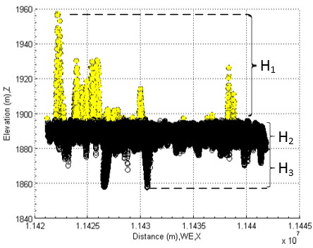 | Figure 19. Select objects over water body of lake |
As seen from it, in terms of different elevations, the detected objects can be grouped into three parts. The first part with elevation H1 obviously does not belong to the water body of lake although they are waters too. The second part with elevation H2 belongs to the main water body of lake. The third part with elevation H3 is one part of water body, but it is below the level of main water body. Three parts are easily discovered by the cross-sectional view. At next stage, the classified parts must be verified by the top view in a two-dimensional remote sensing image.At first, the first part coloured by yellow in Figure 19 is transferred into the imagery in Figure 15 and displayed like the one in Figure 20. From Figure 20, it can be discovered that some edges and spots coloured by yellow is adjacent to water body. In comparison with Figure 15, it can be concluded that water at those zones is located at higher place. Because a remote sensing imagery is made by satellite from space, the water located at high places are then “dropped” onto ground and become one part of water in lake. 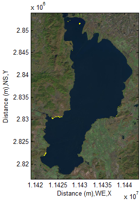 | Figure 20. Detected edges and spots outside lake |
This discovery actually is very important. It points out a potential fatal error for users who use the bottom albedo-independent bathymetry to map the depths of water body. This potential risk is also extended into the commercial package such as ENVI®(Toolbox: SPEAR Relative Water Depth)because SPEAR Relative Water Depthis also based on the bottom albedo-independent bathymetry algorithm. This algorithm completely does not have ability to deal with this unexpected case because all bands were already received by satellite and stored into remote sensing imageries individually. Thus,That may cause the water locating at the high level places to be one part of the water body in river or lake if use this algorithm.
2.10. Verify Location of Main Water Body Based on Elevation of Water
Similarly, the main water body shown by pink colour in Figure 21 must be verified as well. As seen from Figure 22, the main water body located at the middle level is completely represented within the lake except for the discovered edges and spots whose vertical levels are over the ones of the main water body surface and the spots locating below the middle level of main water body.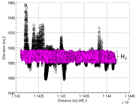 | Figure 21. Select middle layer of water body in lake |
 | Figure 22. Show middle layer of water in imagery |
2.11. Verify Location of Waters underneath Main Water Body Based on Elevation of Water
I, the spots below the middle levels of main water body are able to be displayed in Figure 24 by choosing the third part (coloured by red) shown in Figure 23.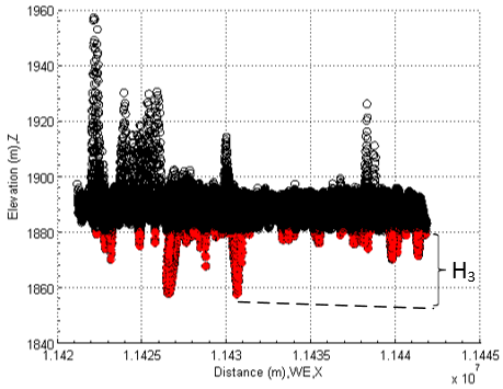 | Figure 23. Select underneath layer of water body in lake |
 | Figure 24. Show underneath layer of water body in imagery |
In fact, this approach is very useful to issue the warning for swimmers or used for other purposes.
2.12. Geometric Feature of a Large Scale Inland Lake
One of important topics in bathymetric modelling is about how the geometric factor of a large scale inland lake affects bathymetric modelling. In general case, for example, a small scale lake in plain has a lower elevation, the shape of bottom could be U-like flat. However, for a large scale lake located at high elevation, the bottom of it becomes very complex and the arc of the earth may have to be taken into account, in this case, α≈0.306944° and β≈0.21665° (see Figure 25), where n is a unit vector normal to any randomly selected surfaces. Thus, it does not have a stable water surface level. 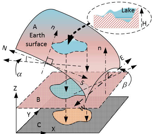 | Figure 25. Geometric feature of a large scale inland lake |
The geometric shape of the lake bottom is more complex. On the one hand, the slope at each spot is different (see Figure 26 and Figure 27), on the other hand, the drop of water surface at different section has a lot of differences (see Figure 28). The full picture of modelled lake is shown in Figure 28. 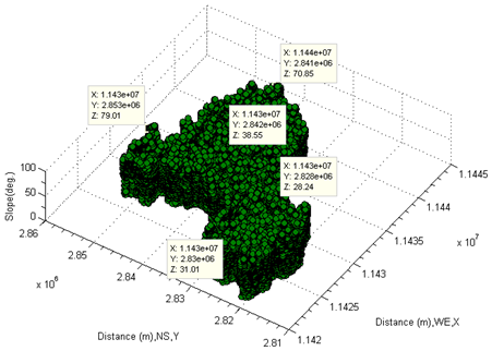 | Figure 26. Show slopes of lake by face-up |
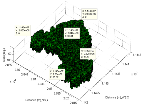 | Figure 27. Show slopes of lake by bottom-up |
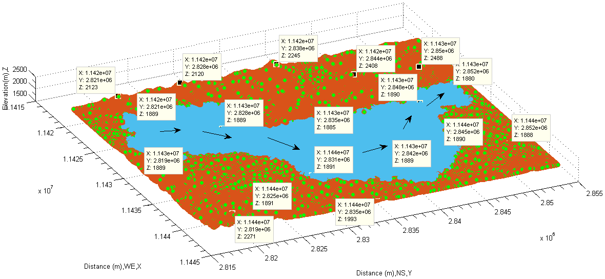 | Figure 28. Overview of water elevation and flow direction |
Above complicated geometric feature indicates that it is extremely difficult to determine the depths of a fully polluted lake using the known methods. Such difficulty in seeking for resolution to it may be appeared by the following imagination. Assume that there were a flat plain or matrix which is able to go through the middle of main water body (see Figure 25, matrix B or Figure 21part H2). That must cause some problems, thus either some volumes of stones at bottom to be parts of body water or some volumes of water to be miss-considered.In other words, there is none water surface which is able to be treated as a horizontal level criterion, and then the depths of water are to be exactly found based on it. It sounds very difficult.In the next subsection, this topic is to be further discussed so as to find a reasonable resolution.
2.13. Obtain Water Depth by Setting Water Body Bottom up
In the last subsection, the main problems in modelling depths of fully polluted water are already pointed out. In addition to them, extra difficulty is that the level of both surface water and bottom of lake is represented as elevation respectively. In other words, to find out the absolute depth of water, setting water body bottom up could be a best way to conveniently handle it. This approach is certainly impossible in reality, but it is not so difficulty to be achieved in MATLAB (the results are to be shown in the last section) by means of special mathematical treatment, thus set the direction of the vertical axis reversely. Discover Pairwise Spatial PointsOnce the water body is set bottom up. The main task is to create a series of pairwise spatial points between water surface and bottom of water body (see Figure 29). For example, when a spatial point a1(x1, y1, h1) at the water bottom (bottom- up side) is found from one figure, the next thing to do is discovering the corresponding spatial point b1(x1, y1, h2) at the water surface (face-up side) from another figure because all of spatial points (a1, b1 and b’1) are projected onto the same spatial point p1(x1, y1, h)which is located on a projected matrix E. On the other hand, the spatial point b1 and b’1are pairwise and exist in the form of symmetry of mirror along the line k1. Where, the h1, h and h2 denotes the elevation of point a1, p1and b1 respectively, the value of h is not required to be sought for. 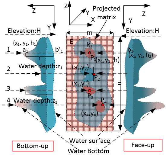 | Figure 29. Find symmetric points at surface and bottom of water body |
Therefore, the depth of water at the point p1 between spatial point a1and b1 can be expressed by the following form. | (18) |
The treatment for other spatial points are similar to above procedure.More about Projected MatrixIn fact, there is an imaginary matrix over the projected matrix E. Each spatial point on the imaginary matrix (named as flexible matrix) has its own Euclidean space, but the case is very similar to the curvilinear coordinates so that each of spatial points is able to flexibly describe very complex shape of water bottom. All of spatial points are projected onto the projected matrix. The imaginary matrix has the same dimension (m×n) as the one which the projected matrix has (see Figure 30) and equals the one which both remote sensing imagery and DEM (thus, 1146×750, in this case) have. The advantage of this approach is that • The complex shape of water bottom factor is completely ignored.• The absolute depth of water body can be found without considering other physical factors out of water.The drawback is that • Each pairwise has to be found one by one manually. 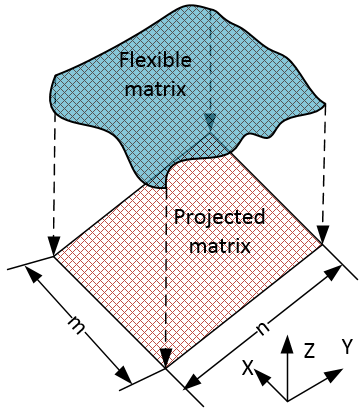 | Figure 30. Flexible and projected matrix |
2.14. Estimate Volume of Water Body
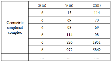
The volume of water body in lake is one of important hydraulic parameters. It can be estimated by the knowledge of computational geometry. In computational geometry [19], an n-polytope P can be dissected into n-polytopesP1, ... , Pk, where the subscript k is an integer. Thus,P = P1∪ ... ∪Pk.Where, the polytopes Pk have pairwise disjoint interiors.Because simplex volumes can be easily computed, a very common approach to computing the volume of a polytope P is to produce a triangulation of Pk. Then compute the volumes of the individual simplices, finally the volume of P is found by summing them up.In topology, a triangulation of a topological space X is a pair (K, h), where K is a geometric simplicial complex and h is a homeomorphism from the underlying space |K| to X.The geometric simplicial complex K is a finite set of simplices in some Euclidean space Rm with m =2, 3. In practice, a three-dimensional Delaunay triangulation is created from the point coordinates in the column vectors, x, y, and z. Then each convex hull and its volume is produced meanwhile (see an example in Table 4).Table 4. Example of convex points to form Delaunay triangulation
 |
| |
|
2.15. Find Perimeter and Surface Area of Water Body
The perimeter and surface area of water body are other necessary hydraulic parameters. The area of surface water (Awater surface) can be estimated by the following relation.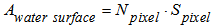 | (19) |
Where, NPixel is the number of detected pixels in lake, Spixel is a unit equivalent area, in this case, it is equal to 32.2000m×32.6963m.The perimeter of water body can be obtained by the conversion between colour digital image and black-white image. Such a conversion is based on the intensity difference of two different colour digital images (see Figure 31). Once such a conversion is achieved, the edge between black and white colours in an image is formed. Such an edge is just a section of boundary between water and land. Then, the sum of the length of each section of boundary is the perimeter of water body in lake. However, the calculating them is in fact one step behaviour if a tool box of image processing in MATLAB is used.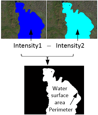 | Figure 31. Generate white-black imagery by means of difference of imagery intensity |
3. Results and Discussion
The results in this section can be grouped into two parts according to the diverse functionality and purpose. In the part one, the concentration is located on finding the hydraulic parameters: depths, surface area, volume and perimeter of water body. In part two, the concentration is on how to find the attenuation coefficient of water using measured absolute depths of water body to verify the quality of polluted water. Eventually, the obtained mean attenuation coefficients of water are used to verify the depths of water body inversely. In a sense, the significance of the reverse verification may be more than the one of the forward modelling. Part 1
3.1. Water Depths
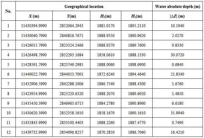
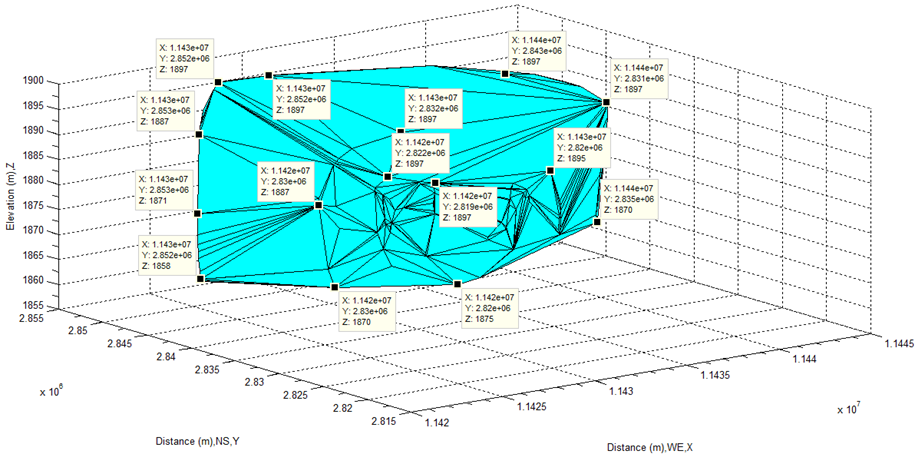
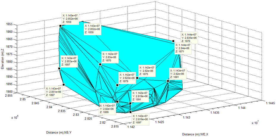
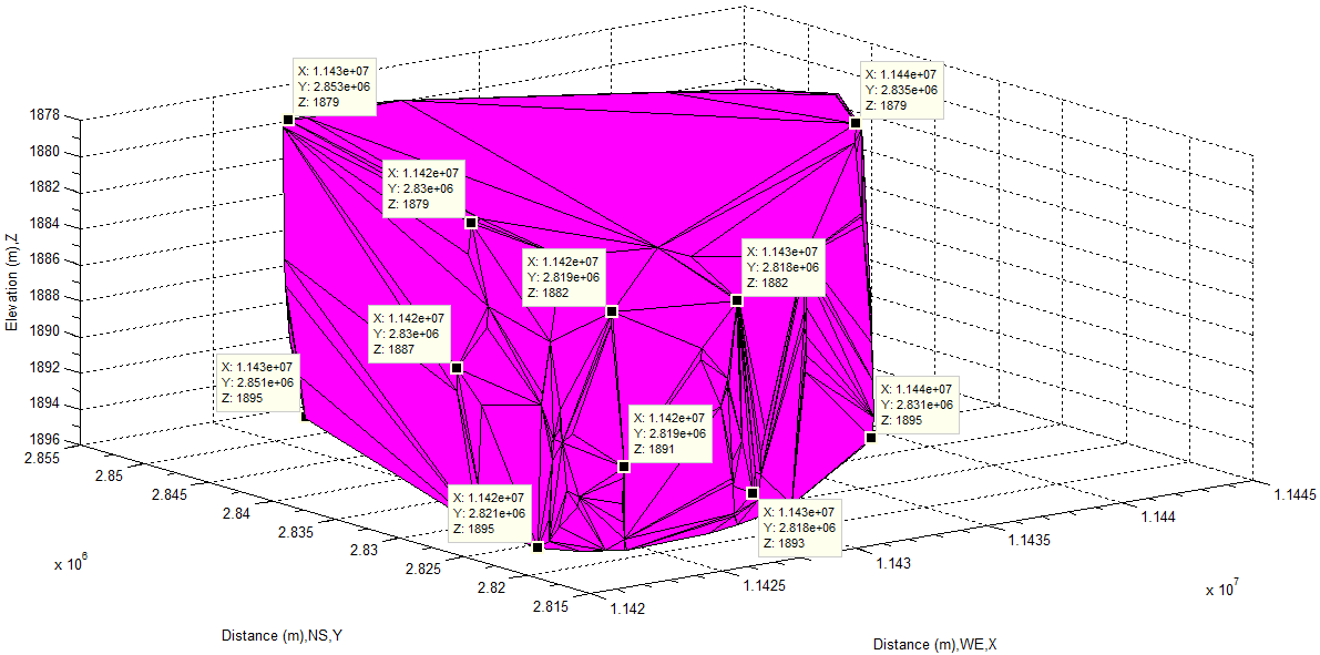
Find Abosolute Water Depths by Difference of Water Elevations In the preceding contexts, the principle of finding absolute water depths of water body is already introduced. In order to obtain the absolute water depths, the data containing elevations of whole water body are represented in Figure 32 and Figure 33 in the form of face-up and bottom-up respectively. A series of pairwise spatial points can be found by combining Figure 32 with Figure 33, however ensure each spatial point have the same two-dimensional coordinates. The pairwise points can be randomly selected. The number of them is only limited to the scale of investigated lake. The data of all spatial points can be stored as a three-dimensional array once the procedure of sampling them is finished. The measured data are already listed in Table 5. Because each pairwise spatial pointsare projected onto the same matrix (see Figure 30), only one two-dimensional coordinates (X, Y) are shown for two corresponding elevations: H1 and H2, each absolute depth (∆Z) of water can be calculated by using equation(18).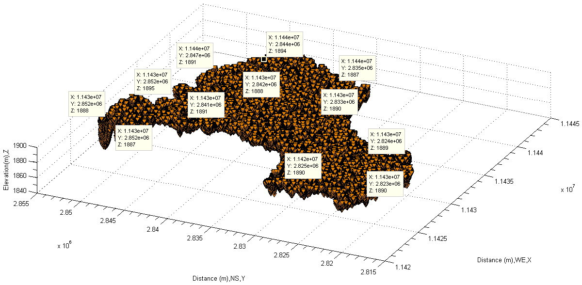 | Figure 32. Show spatial points on the surface of lake by face-up |
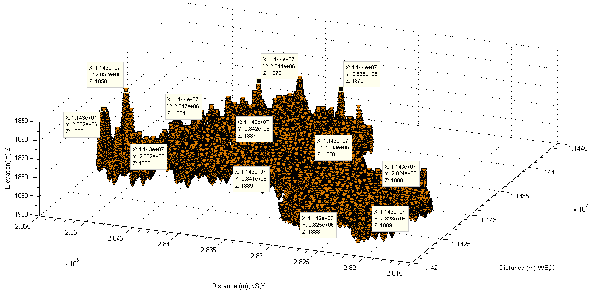 | Figure 33. Show spatial points on the bottom of lake by bottom –up |
Table 5. Discovered absolute depths of lake by using bottom-up manner
 |
| |
|
Actually above procedure can be easily performed by using MATLAB. As mentioned previously, all complex factors can be completely ignored in this approach. The desired data are then easily and accurately gained.Verify Horizontal Locations of Deep Depths of Water from Panchromatic Sharpened ImageryIn reality, the depths of water in lake is impossible to be visualized and verified from the side view. However, there is a simple manner to helpfully verify the horizontal locations of deep depths of water in terms of existing marks on remote sensing imagery so as to prove whether the depths shown by DEM is correct not.In this case, the horizontal locations of the deeper depths in this lake (see Figure 32 and Figure 33) can be seen from the imagery in Figure 34. Figure 34 is a Landsat 8 remote sensing imagery which is formed by using the technique of panchromatic sharpening, hence the individual imagery of band 2 (Blue), band 3 (Green), band 4 (Red), band 5 (NIR) and band 8 (PAN) is pan sharpened. From it, the dark marks denoted by a circle on this imagery are easily discovered. They not only indicate the horizontal locations of deep depths of water but also tell that there are several deep holes there in the vertical direction, which were formed by long term impact of fluid (water) (also see Figure 1) because of the potential and kinetic difference of flow between two different sections in this lake.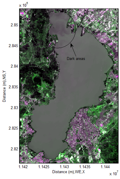 | Figure 34. USGS Landsat 8panchromatic sharpened remote sensing imagery (1146×750) |
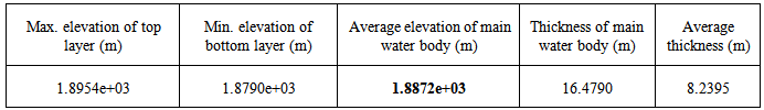
The dark colours in this area are caused by different attenuation coefficient (see equation(11)) while the solar radiation penetrates into those holes from the surfaces of water and reflected from them in the form of scattering. And then their scattered lights travel through atmospheric layer in the form of electromagnetic wave within the visible range (see Figure 4), finally they are detected and captured by sensors installed in satellite.In other words, the distribution of deeper depths shown by DEM in Figure 32 and Figure 33 is correct, and the values of them are then reliable or correct. On the basis of this fact, it can be concluded that whole depths at the rest area of lake are reliable as well. Find Water Depths Using Mean Elevation of Main Water Body In the last subsection, the absolute depths of water are easily obtained by using proposed manner. In order to find reasonable comparison for each different method. Another approach to be shown as follows is based on other calculated data. In Figure 19 and Figure 25, an imaginary flat plain or matrix going through the middle layer of water body used to be considered. However, it does not have result to be represented.In terms of the selected data from the middle layer of water body (see Figure 21), it is easily to find some desired data listed in Table 6. In this case, the average elevation of the main water body (1.8872e+03 meter) is selected as a threshold to classify water body and then the corresponding depths of water are obtained. The results are represented in Figure 35−Figure 37. The negative values means that the depths of water are below the average elevation of the main water body, otherwise they above it. 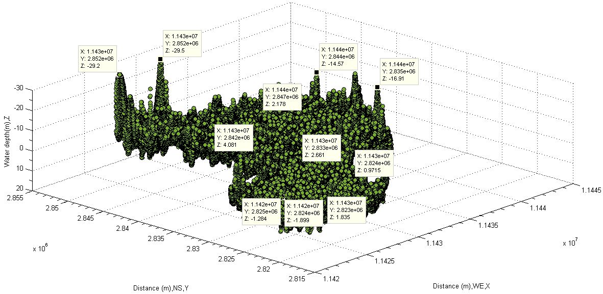 | Figure 35. Depth of lake discovered by using mean elevation of water (bottom-up) |
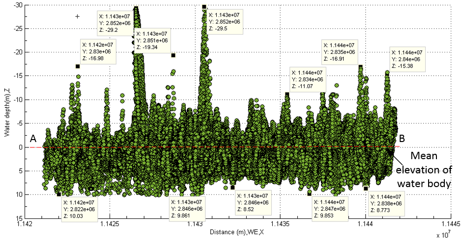 | Figure 36. Depth of lake discovered by using mean elevation of water (side view) |
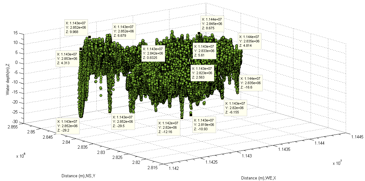 | Figure 37. Depth of lake discovered by using mean elevation of water face-up |
Table 6. Calculated data at the main water body
 |
| |
|
This method in finding depths of water is much quicker than the one introduced in the last subsection. However, the possible drawback is that the selected the average elevation of main water body cannot guarantee that it does not encounter the stone or mud at water bottom when water body is cut off half (see the middle line AB in Figure 36). However, this method may be still useful in handling small scale lake and river with smooth bottom in plain or used into other applications because at least the useful absolute depths can be easily found on the basis of the average elevation of the main water body.
3.2. Water Body Volume
In this subsection, the focus is on finding the volume of water. The mathematic method of calculating it by means of the computational geometry which is already introduced before. However, as it is to be seen, the different treatment in the process of selecting water body is to generate a large difference (error). Thereby the manner of how to choose water body must be taken care of. Calculation by Selecting Whole Water BodyTo perform this task, the first step is to select whole water body as indicated in Figure 38.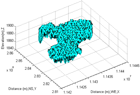 | Figure 38. Select whole water body of lake |
The data selected from three-dimensional coordinates must be verified in two-dimensional coordinates before they are used to calculate the volume of water, otherwise, for example, the waters locating at high levels (if they are not trimmed off) certainly cause a fatal error in the process of calculation. Therefore the examination must be performed at each step. As seen from Figure 39, the area of selected water body is fully located within the original lake (see Figure 15) exclusive of the edges and spots which do not belong to the water body of lake. Finally, the volume of water body is calculated by Delaunay triangulation and shown in Figure 40 and Figure 41. The volume of it is 1.2760e+10 m3 from this calculation. 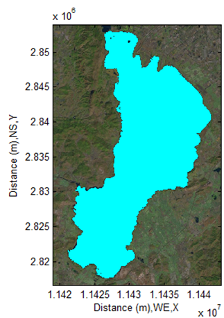 | Figure 39. Show whole selected water body in imagery |
 | Figure 40. Show volume of whole water body by face-up |
 | Figure 41. Show volume of whole water body by bottom-up |
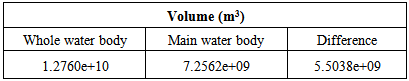
However, this approach of selecting water body seems good enough from the angle of existing water. But a fatal error still remains. The reason can be obtained from further analysis in the following subsection. Calculation by Selecting Main Water BodyAlthough the method used to calculate the volume of whole water body is reliable, mathematically speaking, there is a serious problem which should think of further while using above method. The waters locating at high places are already trimmed off, however, the points locating at the bottom of lake and having a large difference of elevations compared with other points may cause some errors when each polytope is formed. Hence some volumes of mud or stone may be included at bottom level. In order to have a reliable results the deep depths of water should be gotten rid of while performing the calculation of water body volume. Therefore, another approach is to select the main water body only (see Figure 21 and Figure 22).The results using approach is completely different from the last approach. The difference of figures from two calculations is shown in Table 7. The shape of calculated main water body is represented in Figure 42 and Figure 43 respectively. As seen from them, the error of using two different approaches is very large. However, the manner of choosing the main water body is more reliable than the one of selecting whole water body. The reasons are those,1. The surface of water body at surface and bottom approaches to the parallel comparing Figure 42 and Figure 43 with Figure 40 and Figure 41, thus there is not a large amount of mud and stones to be contained in the process of calculation. 2. Several water volume of deep depths of water (see Figure 23 and Figure 24) which are already cut off in the calculation can be compensated by the sum of the small amount of volume of mud and stones. In other words, at least, the partial volume of the deep depths of water is returned to the calculated water volume. Such an error is reduced. 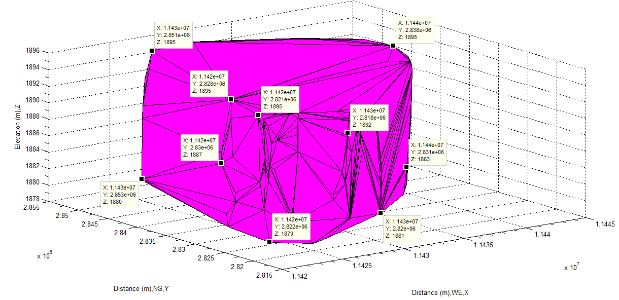 | Figure 42. Show volume of main water body by face-up |
 | Figure 43. Show volume of main water body by bottom-up |
Table 7. Volumes and their difference of the studied lake using two different treatments
 |
| |
|
3.3. Water Surface Area and Perimeter
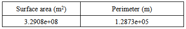
The method of calculating water surface and its perimeter are already introduced in the preceding subsection. The black-white image (see Figure 44) can be generated by selecting two different colours (indicate water body) images, for instance Figure 22 and Figure 39. Then following up the method introduced before, the area of water surface is easily archived. However, the length of boundary have to rely on the image processing tool box in MATLAB. As a brief summary, some modelling results related to the lake besides the depths of water and the volume of water body are listed in Table 8. 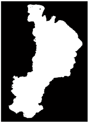 | Figure 44. Obtain water surface and perimeter using black-white imagery |
Table 8. Surface area and perimeter of the studied lake
 |
| |
|
Up to now, the desired values of parameters are already obtained. In the rest subsections, other results related to attenuation coefficients of water are to be employed.Part 2
3.4. Water Quality
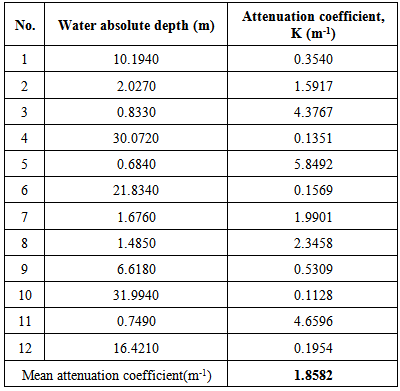
There could be several physicochemical parameters to verify the quality of water in analytical chemistry, however, the quality of water in this research is expressed by the attenuation coefficient when solar light penetrates into the water in lake. According to equation(10), the optical thickness of water has a direct relation with the attenuation coefficient of water. When the water is seriously polluted, on average, the polluted water must have large attenuation coefficient in comparison with the ones listed in Table 1. Attenuation Coefficient Based on Absolute Water DepthsBased on the measured absolute water depths shown in Figure 32 and Figure 33 or Table 5, the corresponding attenuation coefficient of water at each spot is easily calculated by using equation(11) with the data of spectral reflectance (band 3) supplied by MODIS and shown in Figure 18. The calculated attenuation coefficient is listed in Table 9.Table 9. Discovered attenuation coefficient of polluted water using measured absolute depth
 |
| |
|
As seen from Table 9, the attenuation coefficient of water at different spot is different because the concentration of polluted water with other components (thus, pollutants) varies along the direction of flow (see Figure 1 and Figure 28). The mean attenuation coefficient is 1.8582 m-1 in this approach, which is larger than the standard attenuation coefficient of water listed in Table 1 (blue). In other words, the figure indicates that the water in this lake is fully polluted and cannot be used for drinking and cooking. Attenuation Coefficient Relied on Water Surface and Deep Water ZonesAnother approach to get the attenuation coefficient of water is that sampling water takes place close to the deep water zones (see Figure 45). 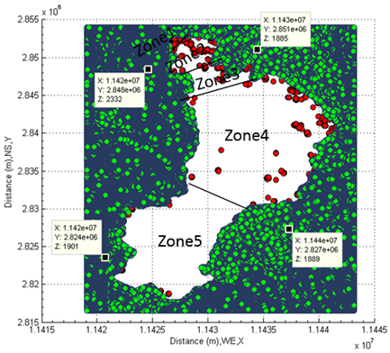 | Figure 45. Sampling zone |
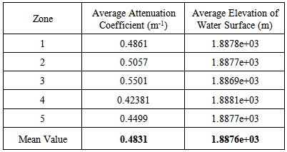
The similar calculation is taken, the data are shown in Table 10. Obviously, and the mean attenuation coefficient is 0.4831m-1, which is smaller than the figure generated by using absolute depths. That is because the sampling happens at places containing deep waters. In short, the attenuation coefficient of water unevenly distributes along the flow direction.Table 10. Average attenuation coefficient obtained by sampling
 |
| |
|
Inversely Verify Water Depths Using Found Attenuation CoefficientsAn inverse problem arises after the mean attenuation coefficients of water being gotten. What do the depths of water look like? If apply known mean attenuation coefficients of water into equation (11). Then, two known mean attenuation coefficients of water listed in Table 9 and Table 10 are used to perform such calculations. The results are shown in Figure 46 and Figure 47. The results are out of expectation.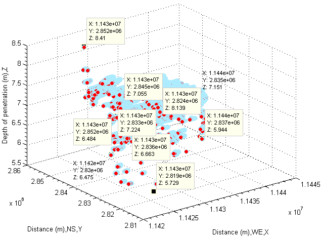 | Figure 46. Depth of penetration using average attenuation coefficient by sampling |
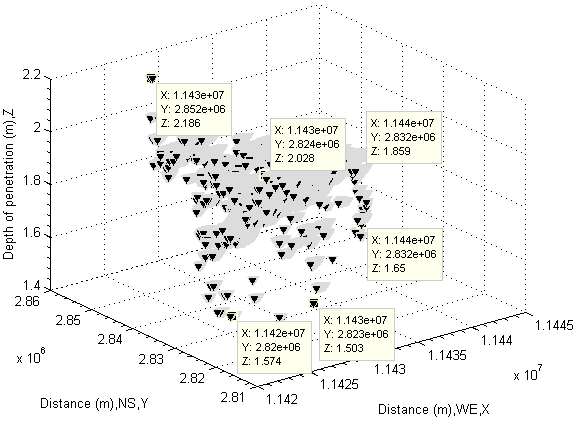 | Figure 47. Depth of penetration using average attenuation coefficient by measured absolute depth |
The depths of water shown by them are smaller than the ones shown in both Figure 32, Figure 33 and Figure 35−Figure 37.Actually, it is not surprised at such results because the mean and unevenly sampled attenuation coefficient of water is used into calculation respectively.However, those results indicate a fact that 1. Detecting depths of water in lake or river by means of sampled attenuation coefficient of water is not reliable especially for seriously polluted water. On the other hand, it is impossible to get an absolute reliable attenuation coefficient because water is fluid flowing at all time.2. It can be further concluded that detecting depths of water in lake or river by means of digital number (DN) recorded by remote sensing imagery may have a similar risk because the different attenuation coefficient produces different DN (intensity) shown in remote sensing imagery.
4. Conclusions
There are many unique features which have been discovered and gained in bathymetrically modelling a fully polluted large scale inland lake and investigating the quality and quantity of its water using proposed methods. The most important issues are summarized as follows and classified into several parts to further discuss against some highly concerned topics including possible doubts.Part 1 Geometry of Water Body and DoubtGenerally speaking, the results of both the distribution of water depths and other desired parameters such as surface area, perimeter and volume of lake are reliable or correct. In practice, they are easily to understand and be proved at the surface level because 1. The horizontal distribution of water depths displayed by DEM can be verified and confirmed by the remotes sensing imagery which is a panchromatic sharpened imagery and clear enough to identify observed objects. 2. The surface area and perimeter of water body are easily calculated by using the technique of digital image processing. However, the main doubt for ones is that whether the data of water depth hidden in DEM and uncovered by the unique technique used in this research is reliable or not, and so on. Because once this matter is confirmed, the volume of water body can be easily calculated and estimated by using the knowledge of computational geometry which has been introduced in this paper.Of course, it is certainly an extremely important topic and highly concerned by ones. To answer such vital questions, it may require more contents. Firstly, as seen from supplied results, the confirmed answer is that 1. A fact of the depths of water in lake or river does exist.2. The data can be discovered by the technique created by author from DEM.3. The discovered data can be displayed. Secondly, as to the question of whether the depths of water body in lake or river is reliable or not, the answer is positive, no matter from the existing fact or theory. The more explanation about depths of water is provided in the following section.Part 2 Explanation about Existence of Water Depths from Process of Generating DEMProviding full explanation to above doubt may be massively in excess of the scope of the current research. However, in order for one to quickly understand the rarely considered topic, the mechanism of forming the data hidden in DEM is only briefly introduced as follows including the historic process of discovering those hidden data, the reasons why they have been ignored for a long time and their significances if they are applied in practice. In fact, such important data were generated by the microwave emitted by the antenna installed at the platform such as USA shuttle or a satellite such as European Remote Sensing satellite (ERS) in the form of pulse. The microwave has longer wavelength which distinguishes from the one used in optical imaging thus remote sensing imaging. Therefore, it can penetrate into many surface of substances reaching to deeper depth. Another difference is that the microwave is emitted in an active manner other than passive manner, so its manipulation is controllable. DEM used in this research is SRTMGL3 or say SRTM3 supplied by NASA (thus NASA Shuttle Radar Topography Mission Global 3 arc second). DEM was generated by using In SAR (Interferometeric Synthetic Aperture Radar). However, in the process of creating DEM, the original synthetic aperture radar interferometric image is flat. The elevation of DEM is generated by the technique called phase unwrapping from two SAR interferometric images, thus make use of the phase difference between two images which are made by platform(s) at different time for the same geographic location.However, a problem is then raised in the process of analysing targets in landscape detected by SAR waves. On the one hand, researchers in radar engineering mainly feel interested in how the wave emitted by SAR transmits in free space and focus on how the backscattered wave is received by the receiver installed in the platform from terrain and the surface of water such as ocean wave. They pay less attention to how the emitted SAR wave impacts upon water body. On the other hand, most GIS (Geographic Information System) researchers do not have much knowledge in engineering, they may be difficult to analyse the mechanism of the backscattered wave emitted by SAR and how it effects water body. Furthermore, an important fact is that such a phenomenon is immeasurable. The reason is to be explained shortly. Because of that, both of them may have been unable to fully discover the existing data of the water body depths, which is already hidden in DEM while it is produced. That could bereas on why any reports about how the microwave emitted by SAR impacts upon the water body hardly have been found in the world so far. The unique technique created and applied into this research by author was used to model large scale bushfire and then model water floodplain (a series of papers have already been published by SAP publishing). However, the outcome from this research is exciting, the elevation of water body hidden in DEM was accidently and successfully discovered. However, interpreting this fact is not so difficult. The scenario is that when the instantaneous powerful external electromagnetic fields generated by SAR wave imposes upon the water body in lake or river (rather than only water surface), the various substances (polar molecules and unpaired charged atoms, most components are water, water H2O is a polar molecule) in it are instantaneously polarized and the transitions of the energy within orbits of polar molecules and unpaired charged atoms then takes place immediately accompanying with the waves are emitted from them in the form of electromagnetic wave. On the other hand, those polar molecules and unpaired charged atoms can affect each other as well and produce extra electromagnetic waves. Their wave lengths may range from IR and radio depending on the strength of external magnetic fields and the strength of magnetic fields generated by the induced polar molecules and unpaired charged atoms. Those electromagnetic waves are also received by the receivers installed in platform. But they fail to have been distinguished from the backscattered wave from the terrain at surface levels. This is another factor causing important data to be ignored by researchers. Once the powerful external electromagnetic fields disappear thus the platform flies away instantly over lakes or rivers, those substances will return to the original random state. However the profile of the elevation of lake or river is then formed immediately by means of above technique thus phase unwrapping. The shape and elevation of geographic structure inside lakes or rivers exactly look like the ones of the visible terrains at surface levels. However, being in mind, water is a fluid, the caves in the bottom of lakes or rivers are completely filled with water (see Figure 32−Figure 37). In other words, strictly speaking, the absolute depths of water body should be the difference between the elevation of water surface and the one of bottom of caves locating at the bottom of lakes or rivers. Such a phenomenon usually is not measurable in site when platform passes over the lakes or rivers in very high speed (e.g.7km/s). Therefore such important data are completely miss-observed by researchers in the world. However, those “ignored” data are extremely vital. As a matter of fact, there are thousands inland lakes and rivers on the earth, nevertheless most of them are lack in accurate bathymetric data. That results in the resistance or failure of development in many diverse relevant fields such as pollution treatment of lake or river, hydraulic engineering, fishing and so on.To fully understand above mechanism of forming data hidden in DEM, it requires specific knowledge in both quantum chemistry, analytical chemistry or physical chemistry and theories of electromagnetics in physics. Actually, on the basis of this secret mechanism, the depth of seawater near coast is also able to be detected and obtained according to the power of modern SAR instead of LIDAR (Light Detection and Ranging), which is too expensive and its application not only is limited but also has error because the wavelength which lasers use ranges from 600 to 1000 nm. NOAA is still using LIDAR to detect the depths of near coast and bathymetric data of Great Lakes according to the report from its official website [20]. It must cost a lot.Unfortunately, such data of DEM near coast fail to be provided by NASA or other space research organizations in the world. That leads to a fact that the depths of seawater near coast fail to be displayed using DEM. The reason why they do not supply them is similar, hence they have realized this fact neither. On the other hand, DEM is based on sea level. Consequently they may not think it is necessary to provide users with those data near coast. In other words, sea-level-based DEM can be extended to near coast area. If so, billion and billion dollars and massive time can be saved in the world.Part 3 Advantage and Drawback of Methods Used in Determining Depths of Water BodyOther advantage of integrating DEM and the corresponding remote sense imagery on which should be emphasised is that the waters positioning at high locations but “melt” into remote sensing imagery by satellite from space when the imagery is made is able to be easily discovered and trimmed off. Such functionality in the technique created by author is unique so as to avoid generating a fatal error especially in calculating the volume of water body in lake or river.The main drawback of the method used in determining the absolute depths of water body is that, because depths of water are shown by DEM in the form of elevation, it is difficult to directly measure them due to the complexity of the shape of water bottom .e.g. in this case. Thereby, author suggests to manually measure them from two separate figures having the same data of water depths according to their same geographic location at horizontal level, thus one is face-up and another is bottom-up. But it is more reliable and much cheaper than finding absolute depths in other manners. In order to find out another manner, the idea is generated in terms of the mean main water body elevation. Thus the absolute depths of water body may be able to be assessed by using the average elevation of the main water body. Because both the waters locating at high position which does not belong to the water body of lake or river and waters which belongs to the water body are cut off in the process of determining he average elevation of the main water body. This manner is much quicker than the first one in handling data. However, the problem is that , based on the average elevation of the main water body, it may encounter the stone or mud at water bottom other than exactly touching the surfaces of bottoms , in other words, the depths of water body may not be absolute if this method is applied into. Nevertheless, this method is still useful in many diverse areas, for example, estimating thickness of water body. Furthermore, in fluid dynamics, it can be used in investigating the trajectory of fluid particle or parcel in the vertical direction if the complexity of water bottom in an open-channel is verified by using bottom-up technique. Or it can be used in measurement in hydraulic engineering. In short, its application is more than author’s imagination. Part 4 Volume of Water Body As seen from the results of volume of water body, how to select water body is extremely important. In this research, the locations of water are classified into three parts in terms of their individual elevation. Although the waters locating at the high places are trimmed off, it still does not have enough reason to calculate the volume of water body by directly selecting whole water body. This is because 1. In the computational geometry, each polytope consists of hulls, however each hull is formed by spatial points (convex points). Then the sum of polytopes is actually decided by a series of spatial points. Therefore how to select those spatial directly affects the accurateness of the result.2. In this case, the bottom of lake is very complicated. The difference of vertical distance between the water surfaces and the deepest cave (water) is more than 30 meters. If all spatial points underneath the main water body are selected and then used into calculating the water volume, that must cause a vital error because a large of amount of mud and stones is included into the volume of water. Therefore, how to select water body relies on the degree of complexity of lake or river. However, in general, selecting the main water body always has less error.Properly choosing water body and then calculating the volume of water body has significant meaning because this technique is also able to be applied into the calculation of storage of reservoirs and other fields. Part 5 Pollution of Water Body As seen from the results of modelling, once several absolute depths of water in lake or river are obtained, the degree of water pollution is easily estimated by using the supplied equation based on Bouguer’s law (or say Beer–Lamber law) integrating the data of spectral reflectance offered by NASA MODIS. In this approach, sampling is quite easy and costs nothing. However, as indicated, the mean attenuation coefficient of polluted water is only used to estimate the quality of water rather than using to measure the depths of water. Otherwise, it certainly causes a large error in seeking for depths of water body.Future ResearchAs mentioned previously, the data of water body depths hidden in DEM has been successfully discovered and displayed. Recently, author has also found similar results or the same phenomena from different lakes and rivers in different countries. In order to fully explain them in detail, author is going to write other academic research paper to further demonstrate this fact which has been being ignored for a long time by other researchers in the world.
References
| [1] | Yoon, Y., et al., Estimating river bathymetry from data assimilation of synthetic SWOT measurements. Journal of Hydrology, 2012. 464–465(0): p. 363-375. |
| [2] | Wang, X., et al., Water-level changes in China's large lakes determined from ICESat/GLAS data. Remote Sensing of Environment, 2013. 132(0): p. 131-144. |
| [3] | Song, C., B. Huang, and L. Ke, Modeling and analysis of lake water storage changes on the Tibetan Plateau using multi-mission satellite data. Remote Sensing of Environment, 2013. 135(0): p. 25-35. |
| [4] | Sima, S. and M. Tajrishy, Using satellite data to extract volume–area–elevation relationships for Urmia Lake, Iran. Journal of Great Lakes Research, 2013. 39(1): p. 90-99. |
| [5] | Duan, Z. and W.G.M. Bastiaanssen, Estimating water volume variations in lakes and reservoirs from four operational satellite altimetry databases and satellite imagery data. Remote Sensing of Environment, 2013. 134(0): p. 403-416. |
| [6] | Legleiter, C.J. and D.A. Roberts, A forward image model for passive optical remote sensing of river bathymetry. Remote Sensing of Environment, 2009. 113(5): p. 1025-1045. |
| [7] | Jay, S. and M. Guillaume, A novel maximum likelihood based method for mapping depth and water quality from hyperspectral remote-sensing data. Remote Sensing of Environment, 2014. 147(0): p. 121-132. |
| [8] | Lyzenga, D.R., Passive remote sensing techniques for mapping water depth and bottom features. Applied Optics, 1978. 17(3): p. 379-383. |
| [9] | Bertoni, R., Linology of Rivers and Lakes in Encyclopedia of Life Support Systems. 2014, UNESCO-EOLSS. |
| [10] | Mobley, C.D., Terrestrial Optics in Handbook of Optics. 2014, Photonics Research Group Department of Information Technology of Ghent University. |
| [11] | Edwards, A., The Remote Sensing Handbook for Tropical Coastal Management. UNESCO, 1999. |
| [12] | Schaaf, C.B., et al., First operational BRDF, albedo nadir reflectance products from MODIS. Remote Sensing of Environment, 2002. 83(1–2): p. 135-148. |
| [13] | Geraldk.Moore, Satellite remote sensing of water turbidity. Hydrological Sciences-Bulletin-des Sciences Hydrologiques, 1980. |
| [14] | DeWitt, F.P.I.D.P., Fundamentals of heat and mass transfer. 2002, New York: Jhon Wiley & Sons, Inc. |
| [15] | Justice, C. and J. Townshend, Special issue on the moderate resolution imaging spectroradiometer(MODIS): a new generation of land surface monitoring. Remote Sensing of Environment, 2002. 83(1–2): p. 1-2. |
| [16] | NASA. MODIS specifications. 2014; Available from: http://modis.gsfc.nasa.gov/about/specifications.php. |
| [17] | Aggarwal, S., Satellite Remote Sensing and GIS Applications in Agricultural Meteorology, M.V.K. Sivakumar, et al., Editors. 2004, World Meteorological Organisation. |
| [18] | USGS. Frequently Asked Questions about the Landsat Missions 2014; Available from:http://landsat.usgs.gov/band_designations_landsat_satellites.php. |
| [19] | Handbook Of Discrete And Computational Geometry. Discrete Mathematics and its Applications ed. J.E. Goodman. 1997, New York: CRC Press. |
| [20] | NOAA. Multibeam Bathymetry 2014; Available from: http://ngdc.noaa.gov/mgg/bathymetry/multibeam.html |
 Abstract
 Reference
 Full-Text PDF
 Full-text HTML