1. Introduction

Every person on the planet lives in a watershed and therefore affects its physical condition. Watersheds vary in shape, area, and characteristics but all watersheds are important to the water cycle. Watersheds are often threatened due to point and non-point source pollutions, drought, and water management conditions. Watershed modeling helps to quantify and define the relationship between land use activities and water quality processes in a convenient and economical way [1, 2]. Hydrologic models integrate information from a wide range of sources into easily-applied decision aids [3]. Furthermore, as [4] point out, “hydrologic models…can be useful to extrapolate estimates of land surface fluxes beyond the resolution of point measurements, provided the land surface characteristics are properly represented in the model”. Using geographic information system (GIS) technology, the accuracy of the models can be vastly improved to account for unique site characteristics that may affect how a particular watershed responds to the activities that are occurring within its boundaries.

There are a myriad of models available today which are capable of simulating the watershed-scale hydrologic processes and yield. Each model has associated proficiencies and limitations, and often the needs of the study dictate which model is most applicable. For this study the Soil and Water Assessment Tool (SWAT) [5] was chosen due to its ability to simulate a broad array of cropping systems and generate reliable estimates of crop yields, and also its ability to estimate the hydrologic response to different cropping and management systems. Crop growth is predominately determined by calculating leaf area development, light interception, and its conversion into biomass. It also considers the accumulation of heat units and once the crop has surpassed the cumulative heat unit required to reach the maturity, growth of the crop ceases [2]. The SWAT can also simulate plant stress that occurs as a result of water, climate, and nutrients. For each time step potential crop yield is first estimated by the defining factors, such as climatic data, crop characteristics, and phenology. The potential is then reduced due to limiting or stress factors, such as water and nutrients. Finally, the actual yield is a result of any reducing factors such as diseases or pollutants. SWAT predicts both biomass yield and yield using the harvest index of the crop, which is defined as the fraction of above ground biomass removal at harvest [2].

The SWAT has gained international acceptance as a robust interdisciplinary watershed modeling tool able to adeptly predict both hydrology and yield [6]. The SWAT has been used for a wide range of environmental conditions, watershed scales, and scenario analyses as described by [6]. The objectives of this study were to: (a) simulate stream flow and soil moisture content variability and (b) quantify corn and soybean yields from the watershed. The models developed from this study can be applied to future studies to assess environmental responses to changes in land use management.

2. Materials and Methods

2.1. Study Area

This study was conducted in two watersheds located in central Mississippi: Town Creek watershed (TCW; 1,775 km²) and a portion of the Upper Pearl River watershed (UPRW; 3,609 km²). The majority of TCW lies within Lee, Union, and Pontotoc counties with smaller portions in Chickasaw, Monroe and Itawamba counties (Fig. 1a). Long-term (1990–2009) records of climate data from Tupelo [7] indicate that that mean annual precipitation is 154 cm with average monthly temperatures reaching a minimum of -19°C in December and a maximum of 42°C in August with a mean annual temperature of 16.3°C. The TCW is primarily designated as cropland [8] with the major water system of Town Creek [9].

The UPRW is located mainly within ten counties (Attala, Choctaw, Kemper, Leake, Madison, Neshoba, Newton, Noxubee, Scott, and Winston) as shown in the Fig. 1b. Long-term climate records (1981–2010) from Carthage [7] indicate that the mean annual precipitation is 142 cm with average monthly temperatures of 17.7°C. The headwaters of the Pearl River begin in the area of the Nanih Waiya Indian mounds and drains in the Ross Barnett Reservoir [10].

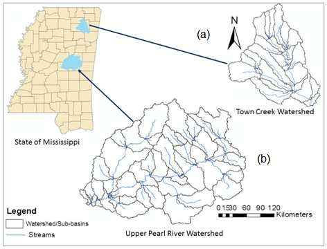Figure 1. Location of the (a) Town Creek and (b) Upper Pearl River watersheds

A total of four fields (Table 1) were chosen as field-scale representations of the UPRW and TCW. All study areas are located on privately owned property and sampling was conducted with the permission of the landowners. In the TCW two crop fields with historical corn-soybean plant rotations were chosen. Field 1 has been harvested the last 30 years with a corn-soybean rotation while Field 2 has historically been a corn-soybean-cotton rotation during the last 20 years. Both locations are adjacent to Town Creek. In the UPRW a representative forest area (Field 3) and pastureland (Field 4) were chosen. Field 3 is a pine plantation that was planted for the first time five years ago and was pastureland before that. Field 4 currently has 10 head of cattle and one donkey that use the area as their primary grazing location. Three points were chosen at each field location at random and labelled as Point 1 through Point 12. Details of the locations and characteristics for each sampling point are summarized in Table 1.

Table 1. Soil Moisture Sampling Points in the TCW (points 1 to 6) and UPRW (points 7 to 12)

2.2. SWAT Model Description

The SWAT was developed in the 1990s by the U.S. Department of Agriculture (USDA) Agricultural Resource Service (ARS) and is based on several other ARS models that were already available [11, 6]. Since its inception the SWAT model has continued to be improved and updated in accordance with advances in knowledge and remains actively supported by the USDA ARS [11]. The SWAT has been used to simulate watersheds around the globe, most often being chosen due to its robust capability to quantify the effects of land management practices on hydrological processes, water quality, and crop growth [5]. There are several versions of the software freely available to the public; ArcSWAT, a version of the SWAT2005 model, interfaced with ArcGIS 9.3 was used in this study. The hydrologic component of the model calculates a soil water balance at each time step based on daily amounts of precipitation, runoff, evapotranspiration, percolation, and base flow. The water balance equation is presented in Eqn. (1) [5, 11].

(1)

where SWt is the final soil water content (mm H₂O), SW0 is the initial soil water content on day i (mm H₂O), t is time (days), Rday is the amount of precipitation on day i (mm H₂O), Qsurf is the amount of surface runoff on day i (mm H₂O), Ea is the amount of evapotranspiration on day i (mm H₂O), Wseep is the amount of water entering the vadose zone from the soil profile on day i (mm H₂O), and Qgw is the amount of return flow on day i (mm H₂O).

Runoff volume for this study was estimated by using the modified USDA Soil Conservation Society Curve Number (SCSCN) method. The SCS CN method depends on the soil cover, management, and soil type. The minimum CN value of 0 implies no runoff, which is not generally possible, whereas the maximum value of 100 implies total runoff [12]. The SWAT model divides a watershed into sub-watersheds, or sub-basins, connected by a stream network. Each sub-basin is composed of hydrologic response units (HRUs) which are unique areas within the sub-basin that account for differences in soils, land use, crops, topography, weather, and slope. The HRU delineation can minimize a simulation's computational costs by lumping similar soil and land use areas into a single unit [11]. Simulations are performed at the HRU level and summarized in each sub-basin. The simulated variables (water, sediment, nutrients, and other pollutants) are first simulated at the HRU level and then routed through the stream network to the watershed outlet [5, 11].

The crop growth sub-model within SWAT is based on the Environmental Impact Policy Climate (EPIC) crop growth model [13]. It is capable of simulating a multitude of vegetation including most crops, some grasses, and forest land [13]. The crop sub-model has several sophisticated features that allow the user to control almost all possible land management strategies and ways plants grow and respond to stresses [6]. For a portion of this study planting date, harvesting date, tillage operations, fertilizer application date and rate were incorporated into the model based on the practices of the landowners at the field sites.

2.3. Model Input

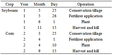
As a physically based hydrological model, SWAT requires multiple sets of GIS data to create data layers to input in the model which control the hydrologic processes in the watershed. Key input datasets include topography, soils data, land use/land cover data, climate data, and management data. U.S. Geological Survey (USGS) 30 meter by 30 meter grids digital elevation model (DEM) data were downloaded and used to delineate watershed boundaries, derive stream networks, and determine slope. The DEM information is a seamless product updated bi-monthly and is a part of the National Elevation Dataset which is derived mainly from 10 meter to 30 meter high resolution, best quality digital elevation data covering the United States, Puerto Rico, and the Virgin Islands [14]. The medium resolution (1:250,000 scale) U.S. General Soil Map (STATSGO) (formerly known as the State Soil Geographic Database) [15] was used to create a soil database for both watersheds. Land use data was obtained from the USDA National Agricultural Statistics Service (NASS). The NASS Cropland Data Layer (CDL) is a raster, geo-referenced, crop-specific land cover data layer with a ground resolution of 56 meters and has 254 recognized land use or land cover categories [16]. Use of this data led to a breakdown of approximately 42 percent forest, 14 percent soybean (annual rotation), and 44 percent other covers in TCW and approximately 69 percent forested, 20 percent pasture, and 11 percent other covers in the UPRW.

The climatic data inputs required by SWAT are precipitation, maximum and minimum temperature, solar radiation, relative humidity, and wind speed. Daily precipitation, daily maximum temperature, and daily minimum temperature data were obtained from the National Climatic Data Center (NCDC) [7] cooperative weather network. Solar radiation, relative humidity and wind speed data, along with any missing observed data, was generated within the SWAT program using the WXGEN weather generator model [17]. This weather generator was developed for the contiguous United States and used for the SWAT simulation studies [11]. Within TCW three weather stations located in Tupelo, Pontotoc, and Verona were used [7]. The SWAT model also used data from the Booneville weather station (part of the U.S. database); this station is located approximately 20 kilometers north of the watershed. The climatic data inputs for the UPRW were obtained from eight weather stations located in Ackerman, Canton, Carthage, Forest, Kosciusko, Louisville, Newton, and Philadelphia [7]. Daily precipitation data for the UPRW were used from all eight weather stations while the daily temperature data were used from only six weather stations (Carthage, Forest, Kosciusko, Louisville, Newton and Philadelphia). The SWAT model used U.S. database data from six weather stations (State College, Russell, Forest Post Office, Meridian, Winona and Canton). The Forest Post Office weather station is located inside the watershed, whereas the other five weather stations are located from 8 to 40 kilometers away from the watershed. Weather station information was assigned to the each sub-watershed based on the proximity of the available stations to the centroid of the sub-watershed [11].

Based on the unique combinations of the input data referenced above, SWAT identified 1,498 distinct HRUs in 31 sub-basins in TCW and 1,916 HRUs in 45 sub-basins in the UPRW. Corn and soybean management data was also input in the TCW model based on information obtained directly from the landowners of the two study fields. Parameters included crop rotation, planting date, harvesting date, tillage operations, and irrigation and fertilizer amount and application dates. It should be noted that the possible sources of errors in model simulated results may come from the model parameters, GIS data used in developing model inputs such as DEM, land use, soils, and weather. Errors due to measured weather data, especially rainfall and temperature, can significantly influence on model results [18, 2].

2.4. Model Calibration, Validation and Evaluation

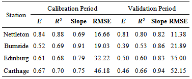
Model performance was evaluated using three commonly used statistical evaluation techniques: the Nash–sutcliffe efficiency index (E), the coefficient of determination (R2), and root mean square error (RMSE) as described by previous studies [19, 19, 20]. Statistical Analysis System (SAS) 9.2 software was further used in some instances to test p-values, and standard correlation calculations.

2.4.1. Stream Flow

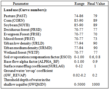
Simulation of the hydrologic balance is usually the first step for all the SWAT watershed applications [6]. Due to the unavailability of field-specific high‐quality input data and theoretical interpretation of hydrological processes, models are calibrated and validated to increase the model’s ability to accurately represent the watershed characteristics [21, 2]. Although the SWAT model was able to perform well in un-gauged watersheds, hydrological calibration and validation was performed using observed stream flow data. Continuous observed mean monthly stream flow data was utilized from the four USGS gage stations (Nettleton- USGS 02436500 in the TCW and Burnside-USGS 2481880, Edinburg-USGS 02482000, and Carthage-USGS 02482550 in the UPRW) in this study.

In this study an un-calibrated, baseline simulation was performed first using SWAT default values for hydrologic parameters. After comparing the baseline model to observed USGS streamflow data, calibration and validation for both watersheds was performed by manually adjusting critical parameter values until maximum model efficiency was achieved when the USGS flow values were compared to model-predicted values at the same location. Manual adjustment of sensitive parameters has been suggested to be the preferred methodology for model calibration [22]. Six widely used flow calibration parameters (Table 2) were selected based on previous studies [6, 23, 24, 18]. The first nine parameters collectively represent the curve number (CN) parameter used for land uses (Table 2). The remaining five parameters in Table 2, are soil evaporation compensation factor (ESCO), base flow alpha factor (ALPHA_BF), surface runoff lag coefficient (SURLAG), ground water ‘revap’ coefficient (GW_REVAP) and threshold depth of water in the shallow aquifer (GWQMIN). The calibration ranges of these parameters were also previously described [20].

Table 2. Parameters, Range and Final Value Used in Model Calibration

2.4.2. Soil Moisture Content

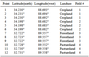
The calibrated and validated model was further used to evaluate the ability of SWAT to predict daily SMC. Observed field data collected at 12 points at four field locations were averaged to yield one value at the 6 inch depth for each sampling date. The SWAT model was run at a daily time step from January 1, 2009 to March 31, 2012 separately for both watersheds, the year 2009 serving as a model warm-up period. Model predicted percent moisture content values were calculated by dividing the predicted SMC value (given in millimeters) by the total length of the soil column (also given in millimeters) and then multiplied by 100. Baseline results were achieved using the previously calibrated models and no further adjustment to parameters was done.

2.4.3. Crop Yield

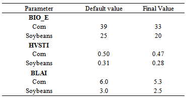
Observed crop yield data was only used in the TCW. Corn and soybeans were the two crops considered based on those being the primary crops within TCW and the crops grown at the two field locations in TCW. County level corn and soybean yield statistics from 1988-2011 were obtained from [25] for the three primary counties that the watershed spans (Lee, Union, and Pontotoc). County level data for corn and soybean yield were weighted by the watershed area in each county to determine watershed scale crop yield. Input parameters that are considered to be most sensitive for predicting biomass or crop yield includes radiation-use efficiency (Bio_E), harvest index (HVSTI), and maximum leaf area index (BLAI) as recommended by previous literatures [26, 2]. The Bio_E, HVSTI and BLAI were adjusted to produce maximum model efficiency when compared with annual NASS yield data. The parameters and their subsequent values are summarized in Table 3.

Table 3. Table of Parameters, Default and Final Values Used in Model Calibration

Field level (Field 2) annual soybean yields data were made available by the one landowner of the study sites for four seasons. Reported soybean yields for the field were compared to simulated yields as well as average yields reported for Lee County where the study site was located. Due to the small dataset, this portion of the study was not a calibration and validation but rather a verification of observed data. Field-specific crop parameters, such as crop rotation, planting date, harvesting date, tillage operations, and irrigation and fertilizer amount and application dates, were defined within the appropriate sub-basin based on information provided by the landowners at the two field sites (Table 4). Fertilizer applied to the soybeans was 00-15-00 at a rate of 200 kilograms and corn fertilizer was 5-15-30 at a rate of 200 kilograms.

Table 4. Crop Rotation and Operations in the Watershed

3. Results and Discussion

3.1. Stream Flow

Four sub-watershed outlets were chosen to calibrate and validate model for predicting monthly streamflow: Nettleton in the TCW and Burnside, Edinburg, and Carthage in the UPRW. These outlets corresponded to locations where USGS gage stations were located. Observed monthly streamflow data were compared to model predicted monthly streamflow outputs. Streamflow was calibrated by manually adjusting critical parameters to improve model efficiency in accordance with the classification established [19]. The TCW demonstrated very good performance for both the model calibration and validation periods (Table 5, Figure 2). Burnside, Edinburg, and Carthage are considered to have shown good performance during calibration. Edinburg maintained good performance during validation while Burnside and Carthage were only fair during validation (Table 6, Figure 2). Likewise, RMSE values demonstrated minimum average error for both the calibration and validation periods for both watersheds (Table 5).

Table 5. Model Efficiency during Stream Flow Calibration and Validation

Table 6. Statistics for Observed and Predicted Values for SMC in all Fields

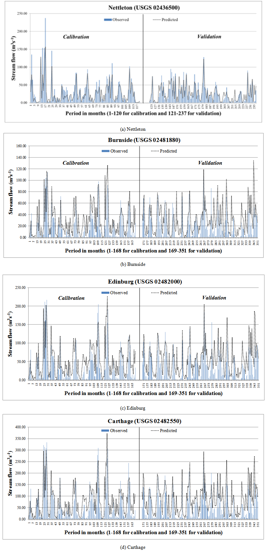Figure 2. Observed vs. Simulated Monthly Stream Flow during Calibration and Validation in the TCW (a) and the UPRW (b, c, and d)

The model performance values of both watersheds is considered to be reasonable in accordance with the scale set forth [19] and is consistent with several studies compiled by [6]. Furthermore, performance of the UPRW model is in agreement with several previous studies [2, 4, 20] using the water models. Based on this it can be said that model performed reasonably well in both watersheds and are assumed to be capable of further predictions of hydrologic parameters such as SMC with minimum bias.

3.2. Soil Moisture Content

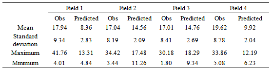
Model simulated daily SMC values from the sub-basin were compared with the field observed SMC values from the field where the sub-basin is located. In all four fields it was determined that the model closely follows a similar curve to observed values, although SMC predictions were consistently under predicted, especially in Fields 1 and 4. Results from a t-test comparing data for Fields 2 and 3 showed no significant difference between observed and predicted values (p = 0.2733 and p = 0.3364 respectively). However, Fields 1 and 4 showed statistically significant under prediction when compared to observed values (p = 0.0015 and p = 0.0008 respectively). Table 6 shows the breakdown of the daily data for observed (Obs) and predicted values for all fields.

In the following graphical representation (Figure 3), the bars on the primary axis represent the daily observed (blue) discrete and predicted (red) daily mean SMC values. Cumulative monthly precipitation (green) is shown on the secondary axis and is given in millimeters. Model predictions were calculated using the baseline calibration and validation parameter values discussed previously. The model clearly demonstrated a similar trend with observed values and more data (at either the daily or monthly time scale) is needed to verify the accuracy of the observed values.

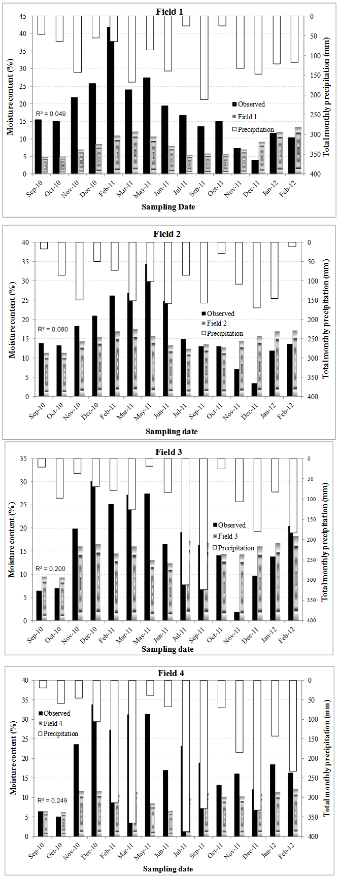Figure 3. Observed vs. Predicted Soil Moisture Content (%) from September, 2010 to February, 2012 for fields 1 to 4

The pronounced discrepancies between observed and predicted values in Fields 1 and 4 could be attributed to physical and hydraulic properties associated with the soils, such as soil texture, rainfall, and hydraulic conductivity, but also land cover and land management practices in place. It is important to keep in mind the scale of SWAT; it predicts SMC at sub-basin scale based on the inputs over the sub-basins or watershed whereas the observed data was being sampled in a comparatively small field area more specifically at point scale. In addition, the critical factors that accounts for the discrepancy was the variation prevalent in the soil sampling techniques (such as local rainfall and time of sampling post-precipitation); soil sampling after a local rain event could have substantially increased the SMC values.

3.3. Crop Yields

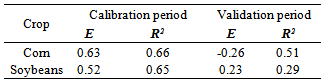
The crop component of this study was performed in the TCW only. The simulated crop yield for corn and soybeans was compared to the county-reported data collected by NASS and to observed data collected from the landowners at the site locations. Simulated crop yield was compared to the county-reported data collected by NASS from 1989-2011 for corn and 1988-2011 for soybeans. When compared with NASS data, SWAT did a reasonable job of replicating annual yields with good statistics (Figure 4) in the TCW (Fig. 1a). Furthermore, E and R2values for both corn and soybeans were within acceptable ranges as reported by previous literature [27, 2] during the model calibration and validation periods for corn and soybean (Table 7).

Table 7. Model Efficiency for Crop Yield

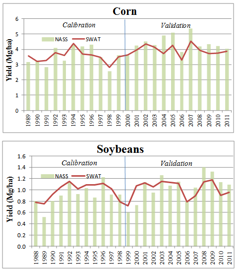Figure 4. SWAT (simulated) and NASS (reported) Crop Yield (Mg/ha) for Corn and Soybeans in the TCW

The SWAT model reasonably predicted soybean yields when compared with the observed data collected from the landowners at the site locations (Figure 5). This finding is important for future simulation because it proves that specific management attributes (such as planting date, fertilization used, fertilizer application date(s), irrigation information, and tillage data) can be specified in the model on a sub-basin level and the model will be able to identify a close range of outcomes based on the changes proposed.

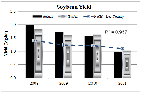Figure 5. Reported and simulated crop yield for soybeans in Field 2 as well as NASS annual average yield for Lee County, Mississippi for reference

4. Conclusions

The purpose of this study was to evaluate hydrologic conditions (stream flows and SMCs) and crop yields from the agricultural fields using the SWAT model. Baseline models were created by inputting required data and delineating the watershed based on topography, soils, and land use. The SWAT model was first calibrated and validated for two agricultural watersheds (TCW and UPRW) using observed monthly stream flow data from USGS gage stations located within the watersheds. Further, model predicted outputs were compared with observed SMCs and crop yields values.

Results from monthly stream flow calibration and validation procedure indicated that model performance was within acceptable ranges as documented in the previous literature [6] based on the classification established [19]. The SWAT model outputs indicate that the model under-predicted SMC of the watersheds by about 32% in this study. Calibration and validation of crop yield predictions in the TCW show close replication of variation seen in reported crop yields from NASS. Similarly, although there was limited data, simulated crop yield from the study locations matched closely with yields reported by the landowner. The TCW can produce average of 3.74 Mg/ha of corn and 1.53 Mg/ha of soybean yields annually. The results of this study could provide essential resource information to watershed managers.

ACKNOWLEDGEMENTS

This material is based upon work performed through the Sustainable Energy Research Center at Mississippi State University and is supported by the Department of Energy under Award Number DE-FG3606GO86025; Micro CHP and Bio-fuel Center. We acknowledge the contributions of Jeffery Hatten in the Dept. of Forestry at Mississippi State University and landowners of the research fields in the watershed for this research.