Nagia E. Elghanduri
Chemical Engineering Department, University of Tripoli, Libya, Engineering College
Correspondence to: Nagia E. Elghanduri, Chemical Engineering Department, University of Tripoli, Libya, Engineering College.
| Email: |  |
Copyright © 2012 Scientific & Academic Publishing. All Rights Reserved.
Abstract
Mass and momentum exchange across a fluid/porous interface is a generic research topic, which also applies to other natural systems such as coastal beaches and aquatic vegetation, as well as manufactured structures such as beach-protection structures and nuclear pebble reactors. The aim of this study is to improve the knowledge and understanding of mass exchange between turbulent flows and their permeable beds by using the computational fluid dynamics (CFD). The focus is on the migration of a passive tracer in the flow fields generated due to turbulence, and flow heterogeneity. Different tracer injection scenarios are studied to investigate mass exchange across a fluid/porous interface by running a series of virtual tracer tests involving the simulations of a passive tracer migration in two-dimensional flow fields generated using Fluent software. Further, it also includes discussion for the effect of the bed porosity on tracer movement using different injection locations. This study succeeded to give a close and detail picture at tracer migration through and over a permeable bed for fully developed turbulent flow.
Keywords:
Tracer, Pulse Injection, Porous Zone, Free Stream
Cite this paper: Nagia E. Elghanduri, Analytical analysis for Tracer Tracking within and over Permeable Bed: Different Injection Scenarios, American Journal of Environmental Engineering, Vol. 3 No. 6, 2013, pp. 273-282. doi: 10.5923/j.ajee.20130306.02.
1. Introduction
In our modern industrialised society natural rivers are under constant threat from pollution. The United State Environmental Protection Agency (EPA) reported in 2009 that 44% of 3.5 million miles of rivers, and streams are impaired or not clean enough to support their designated uses, such as fishing, and swimming[1]. Some of these pollutants are newly spread, others, have been released to the environment a long time ago, and settled on the riverbeds. Once the contaminants are settled, they can act as a source or contaminant reservoir and be released back to the water stream. Understanding and predicting flow and mass transport in natural rivers is therefore very important for their protection. Further, studying the flow through a permeable bed at the bottom of the streams or rivers is very important for understanding the process by which a porous bed acts as a sink for harmful toxins and fine sediments. It is also an ingoing effort to quantify oxygen transport within a pervious streambed with which is important for living creatures in rivers. Previous study be[2] found that the turbulence distributes fine organic particles evenly throughout the water column and increases the opportunities for benthic organisms to capture food. Moreover, the interaction between surface and subsurface water has a crucial influence on the biochemistry of stream environments. When a pollutant or any other substance is released from a point source into an open channel, it creates a plume, which moves in the principal flow direction. Close to the source, the cross-sectional area of the plume is small. It gradually increases with distance from the source due to turbulent dispersion, and/or molecular diffusion until the lateral mixing is complete, and the tracer has spread across the entire cross-sectional area of the channel. The region close to the source can be referred to as a “near field” and the region after the lateral mixing has been completed can be called “far field”[3]. In this study, the tracer migration in the near field is simulated by using point sources for the tracer tests. For straight uniform rectangular-cross section channel of fully developed turbulence, the secondary currents are negligible. The solutes transport in the longitudinal direction. In the longitudinal direction solute transport due to diffusion turbulence, and vertical velocity gradients. Further, the spreading caused by the variations in velocity and concentration in the transverse direction is neglected. However, within the porous zone, the flow is heterogeneous, and the transverse flow currents play important role.Solute transport after two lumping steps can be described by the following two-dimensional equation: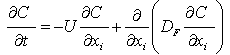 | (1) |
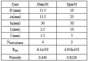
Where C, is the spatial averaged concentration, U is the time and spatial averaged velocity, xi is the tested flow Cartesian coordinate, and DF is the local depth averaged transverse mixing coefficient[4].The objective of this study is to investigate mass exchange across a fluid/porous interface by running a series of virtual tracer tests involving the simulations of a passive tracer migration in two-dimensional flow system that consists of a boundary layer and an adjacent porous layer. This study is two-dimensional CFD analysis made for two different porosity cases with the same geometry data for previously published data by[5]. Two systems with identical boundary layer thickness but with different porosities, namely dens30 and spar30, were selected for this analysis. The geometric and hydrodynamic for these two cases are presented in Table 1 and the geometry symbols are sketched in Figure 1. Migration of a tracer in these flow fields was simulated using the Discrete Phase model. The Discrete Phase model is a numerical tracer tracking model that included in the software Fluent. It tracks tracers up to concentration 10%. Different injection scenarios are set up in order to investigate the tracer movement within and over porous layer, which corresponds to a variety of (idealised) real world cases.Table 1. Geometric and hydrodynamic characteristics of the simulated cases[5]. The meaning of different symbols is shown in Figure 1. Geometric and Hydrodynamic Characteristics
 |
| |
|
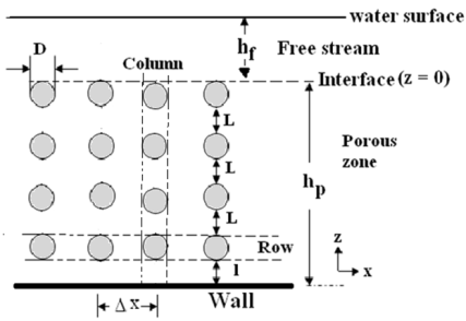 | Figure 1. Columnsand rows of the arranged rods bundle and symbols for geometry |
2. The Studied Cases
The studied cases were for flow over and within a porous zone. The porous zone was rods mounted horizontally. Two distinctly different cases are compared and contrasted: (i) the sparse case (spar30) with a sufficient space between the obstacle for turbulence from the free surface zone to penetrate deep into the porous layer; (ii) dense case(dens30) with very small gap between the obstacles, characterised by distinct recirculation vortices at the downstream side of each obstacle and with very shallow penetration of turbulence, which does not go beyond these vortices. The pre-processor was Gamibt where the geometry of cases were built in and meshed. The numerical simulation was done by Ansys in Fluent software. The simulation was for fully developed turbulent flow region within both free stream and the porous zone. A large flumes where built to achieve the fully developed turbulent zone which consumed a large simulation time. The simulation was run for steady state until turbulent fully developed turbulent flow zone is reached. The simulation results were verified with previously published results at[5], and[6] at the fully developed turbulent zones. A good agreement was achieved for comparing the normalized turbulent kinetic energy (TKE+), and the velocities (U+) versus normalized bed height for a mid-line between two column rods as shown in both[7] and Figure 2.The injection process was carried out at the fully developed turbulent flow region in both free and porous zones for all tested cases.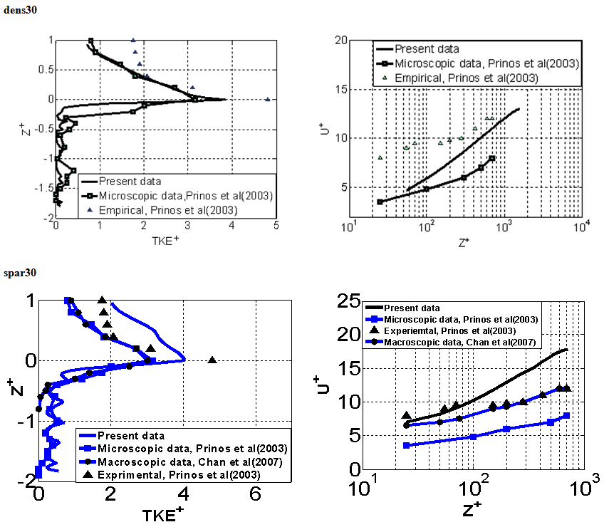 | Figure 2. Comparison between previously published and present study for normalized turbulent kinetic energy profile above and within porous medium (left), and normalized velocity distribution at the free stream(right) for the simulated cases |
3. Injection Scenarios
The tracer injection was unsteady state process for both simulated cases. The tracer tracked using Discrete phase model. The discrete Phase model is a numerical model included in Fluent software for tracer injection and tracking. In general, the discrete Phase Model (DPM) is used if the mass flow rate is less than 10% of the total mass flow rate[8]. A series of point injection tracer tests have been carried out. The simulation was for both cases using software Fluent in Ansys12 as mentioned previously. All simulations start at time t = 0 and the tracer is injected into the pollutant-free system so the initial tracer concentration is zero. The tracer injection velocity is always equal to the velocity at the source. To avoid buoyancy effect the tracer density is set the same as water density. The total simulation time is 3 seconds, with a time step of 0.01 seconds. Regarding the duration of injection there is a short test so-called “pulse injection” (duration 0.1s). The raw simulation results consist of a time-series of concentration fields, where each field is defined by a series of values for concentration across the simulation domain at a given time, i.e. by C(x, z, t). The position of the source was varied between the tests in order to cover all relevant flow regions. All source positions are shown in Figure 3. The injection point in the free stream (FS) is situated at the midpoint between the water surface and the interface. The interface injection point (I) was located at the level of the top of the highest rods in the middle in between two rods. Several further points are located within the porous zone as shown in Figure 3. The mass of tracer injected was about 0.7 (Kg/s) for all injection scenarios in both tested cases. This amount of tracer was selected by trial and error. It is large enough that it can be tracked within the bed, but small enough to not affect the flow velocity. Figure 5 shows an example of the simulation results in form of the contours of tracer concentration after a pulse injection at point T1 for the sparse case. These concentration contours indicate that tracer tends to move along the same gap between the rod-rows, and also to spread in the longitudinal and lateral direction.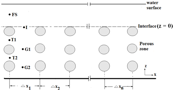 | Figure 3. Sketch locations of injection sources in the free stream (FS), at the interface (I) and in the porous zone (T-point at a pore throat, G-point in the gap between the cylinders) |
The simulated variables from Fluent were available to large number of spatial points for different time intervals. Further, they were heterogeneous. In order to obtain macroscopic data, averaging technique was applied for each time instance. A computer program was built using Matlab software to read the exported data and average it. The values for concentration were averaged over thin slices parallel to the principal flow direction (x-axis), and spanning the centre-to-centre distance between the rod columns (Figure 4). The result of averaging is assigned to the centre of the averaging volume. This produced a time-series of different tested profiles such as vertical concentration profiles (xi, z, t), longitudinal velocity profile, x>(xi, z, t), at a series of x-positions of averaging volumes, denoted with xi (i= 1, …., 10). Alternatively, the instantaneous concentration fields were averaged over large areas covering the height of either the free stream or the porous layer, and spanning the centre-to-centre distance between the rod columns (Figure 4). Resulting average concentrations and velocities are denoted with (CF,Uxf), and(Cp,Uxf) for the surface, and porous zone respectively.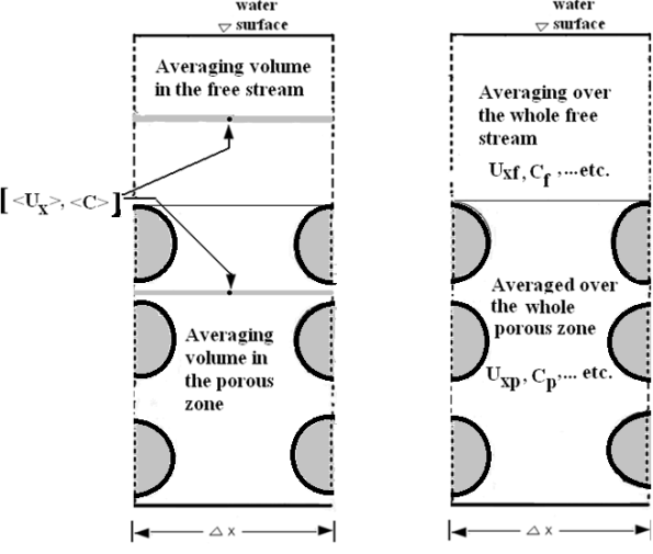 | Figure 4. Schematic diagram illustrates the averaging volumes; left plot illustrates averaging over thin bed-parallel volumes: the right plot illustrates averaging over the whole free stream and the whole porous zone |
The following sections present the results of the tracer tests, followed by the evaluation of the parameters, which quantify the large-scale tracer migration and the mass exchange between the free stream and the adjacent porous layer.
3.1. Free Stream Injection (FS)
Migration of tracer after a pulse injection at the FS point (Figure 3) is recorded using break-through curve plots at various x-locations downstream from the source (Figure 6). The distance of the centre of the control volume ∆xn from the source is 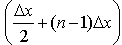 . The break-through curves for sparse case have Gaussian shape typical for dispersion in open channels. Numerous studies published similar pattern for experimental results such as[9], and[10] among others. The exception is the x-location which shows a double peak, indicating two principal advection velocities instead of one. The second peak is visible to some extent for ∆x7, and is quite distinct for ∆x9. Two different advection velocities probably belong to the faster and slower part of the velocity profile. Initially the track plume is located in the middle of the flow depth and the tracer moves at the same speed. Later on, the plume becomes thicker due to the lateral dispersion. The upper part of the plume moves considerably faster than the lower part, resulting in the double peak in the break-through curve. This phenomenon is much more pronounced for the dense case, where all break-through curves have multiple peaks.
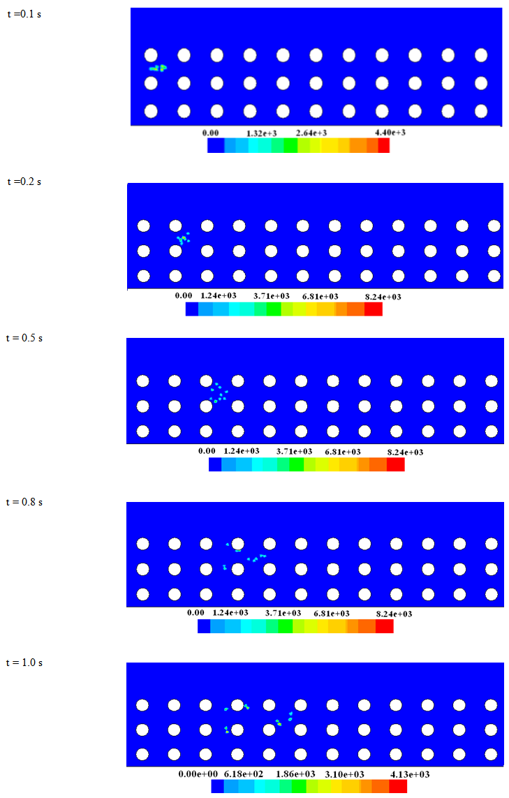 | Figure 5. Contours of tracer concentration (Kg/m3) after a pulse injection at point T1 for the sparse case |
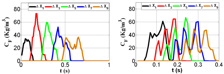 | Figure 6. Tracer distribution within the free stream for point injection (FS) for spar30 (left), and dens30 (right) |
3.2. Interface Zone Injection (I)
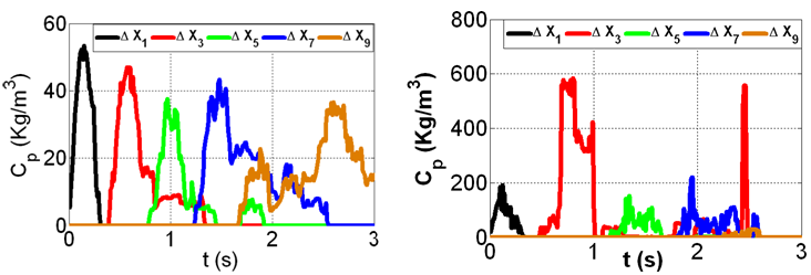
The break-through curves for both free stream and porous zone are shown in Figure 7. The interaction between free stream and porous zone is clearly visible for the sparse case. The tracer appears in the porous zone when it has disappeared from the free stream zone and vice versa. This movement between the zones occurs several times during the simulation.Further, the tracer concentration in sparse case within the free stream is nearly doubled that in the porous zone. For the dense case, the tracer remains in the free stream much longer and has higher concentrations compared to the sparse case. This is due to both the smaller distances between the rods compared to the sparse case, and the presence of stationary vortices within the interface zone[7]. Tracer is therefore trapped within the circular flow pattern so it accumulates with high concentration values. This flow pattern delayed the tracer migration to the porous zone compared to the sparse.Figure 8 shows the average tracer mass pass through Δx2 zone (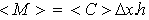 ) within both free stream (h=hf) and porous zone (h=hp) vs. dimensionless time. The dimensionless time is computed as t* = t U/x where U is average velocity throughout the flow column (U =Q/(hf+ hp)), where Q is the discharge. This Figure shows that the tracer injection within the interface penetrates to the free stream faster, and in larger amount in both tested cases. Furthermore, the residence time within the contour volume ∆x2 is much longer for the dense case, which has distinct recirculation vortices close to the interface level, which trap the tracer and hence increase residence time.
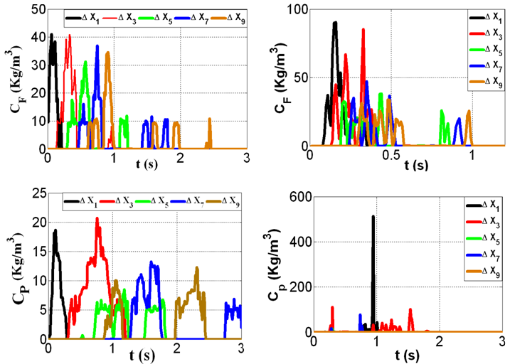 | Figure 7. The tracer averaged concentration change with time for interface point injection (I) at both free stream(top), and porous zone(bottom), for both spar30 (left), and dens30 (right) |
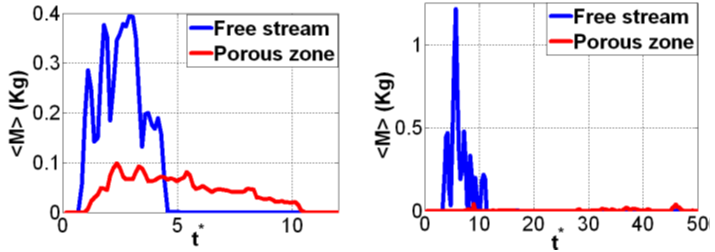 | Figure 8. Mass of tracer within ∆x2zone versus normalized time in both free stream and porous zone for spar30 (left), and dens30 (right) for interface injection scenario |
3.3. Injection in the Vertical Gap between the Rods (T1, and T2)
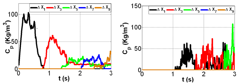
Figure 9 shows the break-through curves at different x-locations for the injection source located at T1 (Figure 3). For the sparse case, the tracer concentration close to the source shows a pattern similar to that for the free stream. The pattern deforms at the further distances from the source. The deformed shape is probably due to tracer deposition in the recirculating vortices behind the rods, which delays the tracer migration. Furthermore, the tracer may return to the upstream zone. The tracer movement in the spar30 case has much more stable pattern compared to the dens30 which reaches very high concentration values at some bed locations. This indicates that at some locations plenty of tracers get trapped between the rods.Figure 10 shows the break-through curves for T2 injection. Their pattern is very similar to T1 injection. However, concentration values for T2 are lower.Figure 11 shows the break-through curves for injection from point G1 (Figure 3). As before the curves for the dens30 have very different pattern than the spar30 curves. The tracer in the dense case is moving with very low velocity, it could not enter the last tested x-location within the tested time. Furthermore, the break-through curves are very scattered. This may due to the presence the vortices at the upper and the lower sides of the rods. The tracer therefore gets trapped between the rods, part of it moves in circular movement with the vortices, and the rest of the tracer moves with the flow. The break-through curves for the sparse case are much smoother. The maximum concentration occurs at x1 because further downstream begins vertical spreading. The tracer enters the downstream locations with a lower concentration and stays there longer time. Between further locations, the tracer concentration curves show slower movement which indicates that lateral spreading of tracer affects its longitudinal speed, and since the tracer moves with higher velocity at the lower part of the bed (discussed in[11], and[7]). For the dens30 case, the difference in concentration values between various x-locations is smaller, as the higher velocity prevents some of the tracer from getting trapped between the rods, compared to T1 source. Figure 11 shows that close to the source location breakthrough curves have a smooth Gaussian shape, which indicates that, the tracer moves at pore velocity. However, further away some tracer gets trapped between the rods. This delays tracer migration from that zone to the downstream locations resulting in more ‘peaky’ breakthrough curves.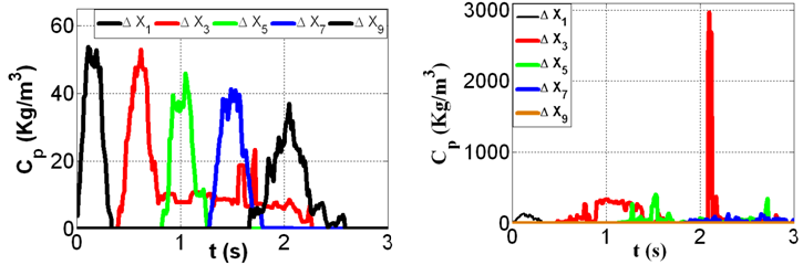 | Figure 9. Tracer averaged concentration change with time at different locations within the porous zone for point injection T1; spar30 (left), and dens30 (right) |
 | Figure 10. Tracer averaged concentration change with time at different locations within the porous zone for point injection T2; spar30 (left), and dens30 (right) |
 | Figure 11. Tracer averaged concentration change with time at different locations within the porous zone for point injection G1; spar30 (left), and dens30 (right) |
3.4. Injection in the Vertical Gap between the Rods (G1, and G2)
Figure 12 shows the break-through curves for tracer injection from G2. The tracer movement is very similar to that for G1, especially close to the source. However, the accumulation between the rods for the dense case is more pronounced resulting in higher values of concentration than for G1 injection.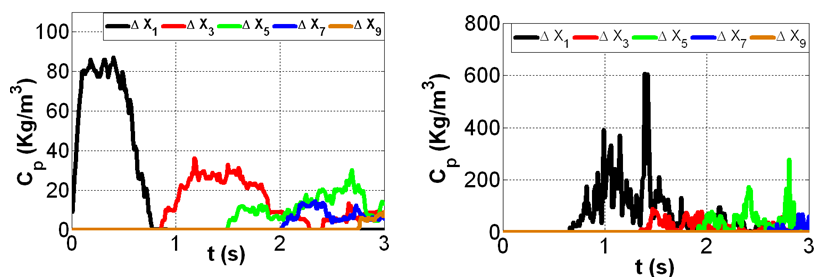 | Figure 12. Tracer averaged concentration change with time at different locations within the porous zone for point injection G2; spar30 (left), and dens30 (right) |
4. Effect of Source Location on Tracer Distribution within the Porous Zone
Within this section, the source location effect will be discussed only for the porous zone, where the flow is more heterogeneous. Figure 13 shows the breakthrough curves for the four injection points within the porous zone. It can be noticed that despite the same type and amount of tracer, as well as the same stream flow conditions, there are differences in tracer spreading from different injection places. This is due to the difference in the spatial structure of flow. Overall the plots for both cases (Figure 13) show that tracer migration from T1 is similar to that of T2, and from G1 is similar to that of G2. This similarity is due to the similar flow conditionsdownstream from G1, and G2, as well as T1, and T2. Close to the source location, a larger tracer amount in G injection is noticed compared to T injection scenario. Furthermore, at farther distances the tracer movement from T1 source shows a delay compared to T2. This is because of the higher velocity in the lower part of the bed compared with that close to the interface. Further, Figure 13 shows that source location has an important effect on the tracer distribution within the porous zone. Further, the interaction between the free stream and the porous zone takes a long time and hence occurs beyond the tested zones, which indicate that the longitudinal dispersion within the porous zone is much larger than the lateral dispersion. So, the source location effect will be discussed only for the porous zone, where the flow is more heterogeneous. The breakthrough curves for the four injection points within the porous zone. It can be noticed that despite the same type and amount of tracer, as well as the same stream flow conditions, there are differences in tracer spreading from different injection places. This is due to the difference in the spatial structure of flow. Overall the plots for both cases show that tracer migration from T1 is similar to that of T2, and from G1 is similar to that of G2. This similarity is due to the similar flow conditions downstream from G1, and G2, as well as T1, and T2. Close to the source location, a larger tracer amount in G injection is noticed compared to T injection scenario. Furthermore, at farther distances the tracer movement from T1 source shows a delay compared to T2. This is because of the higher velocity in the lower part of the bed compared with that close to the interface. Further, Figure 13 shows that source location has an important effect on the tracer distribution within the porous zone.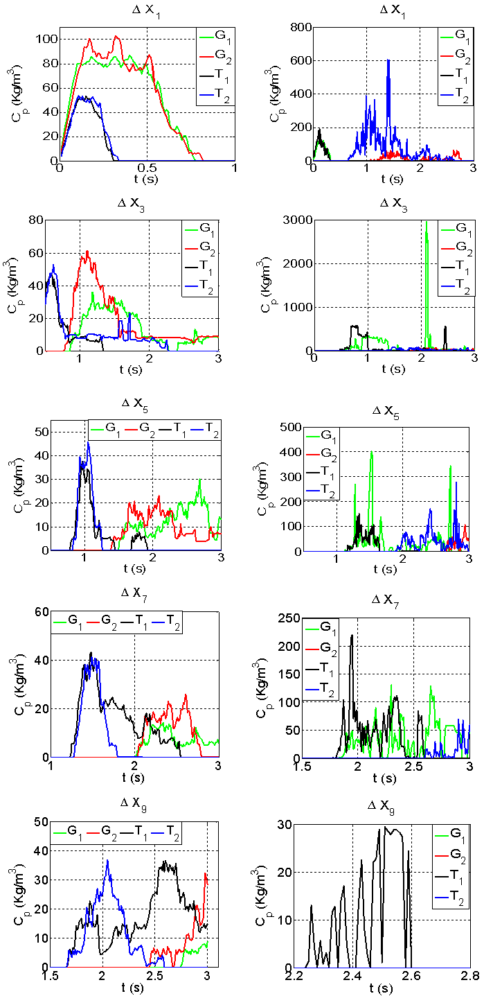 | Figure 13. Break-through curves at different locations for spar30 (left), and dens30 (right) |
5. Conclusions
This study provided close insight into the tracer dispersion in fully developed turbulent flow over and through a permeable layer.Rapid releases of a limited mass of tracer, called pulse injection for series of locations of point tracer source have been tested. The contour plots of the tracer concentration are presented in order to provide visual information of the tracer pathways. Spatially averaged results in the form of concentration profiles at various time instances and breakthrough curves for various locations provide more concise information, which allows a quantitative analysis. The analysis includes the influence of porosity of the permeable layer on the tracer migration and fluid/porous exchange, as well as the temporal and spatial statistical moments. The main conclusions from the analysis are:● Following a pulse injection across the whole of the free stream thickness the exchange with the porous zone occurs faster for the sparse than for the dense case. On the other hand for the dense case the tracer moves through the free stream faster and remains within the porous zone longer, compared to the sparse case. ● When the tracer is injected from a point source located at the interface it moves in the streamwise direction and also spreads in the lateral direction, hence penetrating both into the free stream and into the porous layer. However, the lateral spreading is asymmetric, resulting in the majority of tracer moving within the free stream. Due to a better contact between the free stream and the porous zone the asymmetry of the lateral spreading is much less pronounced for the sparse case than for the dense case. As a result the masses of tracer moving in the free stream and in the subsurface for the sparse case are comparable, whereas for the dense case practically all of transport occurs in the free stream. In either case the dispersion within the porous layer is much more pronounced than in the free stream.
References
| [1] | I. Javandal, C. Doughty, C. Tsang "Ground water transport: Handbook of mathematical models ", American Geophysical Union, Water Research Monograph, 1997. |
| [2] | A. Malcolm, C. Soulsby, A. Yougson, D. Hanah, I. McLaren, (2004) "Hydrological influences on hyporheic water quality: Implications for salmon egg survival"Hydrolo. Processes, vol. 18, pp. 1543-1560, March, 2004. |
| [3] | G. Jirka, T. Bleninger, R. Burrows, and T. Larsen, "Management of point source discharge into rivers: where do environmental quality stands in the new EC-water framework directive apply?" Intl. J. Basin Management, vol.2, No.3, pp. 225-233, 2004. |
| [4] | W. Zhang "A 2-D numerical simulation study on longitudinal solute transport and longitudinal dispersion coefficient", Water Resource Research, vol. 47, W07533, doi: 10.1029/2010WR010206., pp. 1-13, 2011. |
| [5] | P. Prinos, D.Sofialdis, and E. Keramaris "Turbulent flow over and within a porous bed" Journal of Hydraulic Engineering, pp. 720-733, Sep., 2003. |
| [6] | H.C. Chan, M. Leu, C. Lai, M., and YafiJia, “Turbulent flow over a channel with fluid – saturated porous bed”, Journal of Hydraulic Engineering, June, pp. 610 – 617, 2007. |
| [7] | N. Elghanduri"CFD Analysis for Turbulent Flow within and Over a Permeable Bed" American Journal of Fluid Dynamics, vol.2, no.5, Oct., 2012. |
| [8] | Manual Ansys 12, ANSYS CFX-Solver Manager, User’s Guide, ANSYS, Inc., January, 2009, www.ansys.com |
| [9] | Bencala, and R. Walters '' Simulation of solute transport in a mountain pool- and- riffle stream: A transient storage mode'', Water Resources Research, vol. 19, No. 3, pp. 732 – 739, 1983. |
| [10] | K. Bencala "Interaction of solute and streambed sediment 2. A dynamic analysis of coupled hydrologic and chemical processes that determine solute transport", Water Resource Research, vol. 20, no. 12, pp. 1804-1814, 1984. |
| [11] | D. Pokrajac, C. Manes, and I. McEwan "Peculiar mean velocity profile within a porous bed of open channel" Physics of Fluids, vol. 19, no.9, -098109-1-5, 2007. |
 Abstract
 Reference
 Full-Text PDF
 Full-text HTML