A. Amr M. Sabry 1, M. Naguib 1, Alya Badawi 1, Tarek Nagla 2
1Nuclear & Radiation Engineering Department, Alexandria University, Alexandria, Egypt
2Nuclear Power Plants Authority (NPPA), Cairo, Egypt
Correspondence to: A. Amr M. Sabry , Nuclear & Radiation Engineering Department, Alexandria University, Alexandria, Egypt.
| Email: |  |
Copyright © 2012 Scientific & Academic Publishing. All Rights Reserved.
Abstract
This paper aims assessing the environmental impact of oil spills which are caused by hypothetical oil tankers and offshore nuclear power plants accidents; where the effect of the changes in wind and water current on the oil spill movement and fate is studied. In case (a), multiple oil spills which are caused by a tanker accident near to the north coast of Egypt in the Mediterranean Sea are simulated by MEDSLIK[1] software. In this case, variable wind data is documented every 24 hours for 10 days[5] of simulation and non-uniform current input[4] were used. In case (b), the best guess[2] of oil spill trajectory and the associated uncertainty of an oil spill occurred on the Iranian coastline in the Arabian Gulf after an accident in Bushehr Nuclear Power Plant, which is caused by an earthquake, are calculated by using GNOME[2] software. In this case, wind forecast data from Bushehr Airport meteorological station[3] and three current patterns[2] are used to simulate the oil spill dispersion. These cases give decision-makers critical guidance in predicting the behavior of oil spills in the studied regions. Moreover, they show the effect.
Keywords:
MEDSLIK, GNOME and Trajectory Analysis
Cite this paper: A. Amr M. Sabry , M. Naguib , Alya Badawi , Tarek Nagla , Assessment and Modeling of Oil Spill Dispersion in Mediterranean Sea on the North East Coast of Egypt and the Arabian Gulf, American Journal of Environmental Engineering, Vol. 3 No. 5, 2013, pp. 236-252. doi: 10.5923/j.ajee.20130305.05.
1. Introduction
Accidental and illegal marine pollution in the Sea water constitutes a major threat to the marine environment. Previous incidents in the Mediterranean Sea and the Arabian Gulf have resulted in environmental and economic damages to fisheries, to the tourist industry and to coastal marine ecosystems. Oil-pollution discharges from ships and offshore power plants in the Mediterranean and Arabian Gulf have been described as significant and are a cause of environmental degradation in the seas of the Middle East region. To prevent the major impact of accidental oil spills, local and regional preparedness and response plans recommend the use of computer-aided support systems based on operational oceanography and real-time ocean forecasts and real-time ocean forecasts coupled with satellites images and oil spill models.
2. Materials and Methods
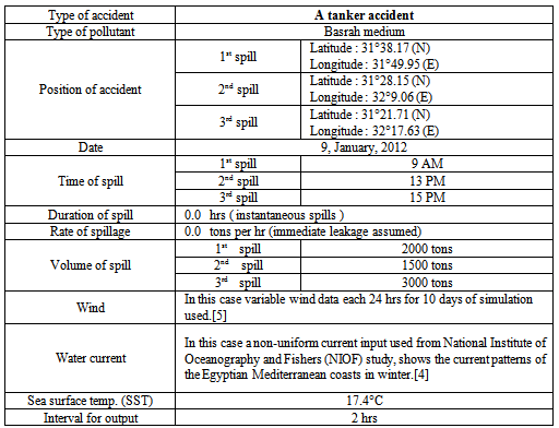
Table (1-a). Input data
 |
| |
|
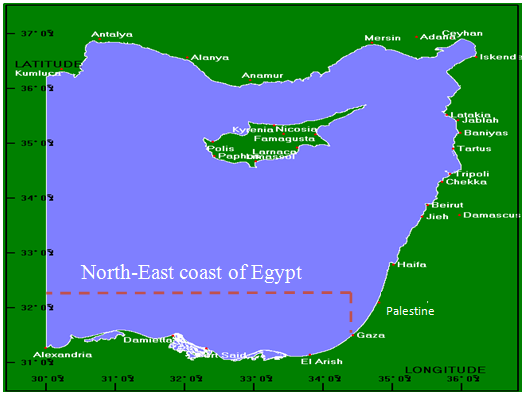 | Figure (1-a). Levantine Basin map by MEDSLIK |
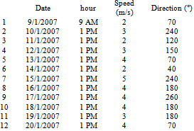
a) MEDSLIK incorporates the use of forecasts developed under MFS (Mediterranean forecasting system) program for the whole Mediterranean Sea and its sub-regions such as Levantine Basin (figure (1-a)). This program was used to simulate a multiple oil spills occurred by a tanker near to the north coast of Egyptian. MEDSLIK uses a modified version of Mackay's fate algorithms for evaporation and emulsification and the dispersion algorithm of Buist and Mackay[1]. The following is the typical data and information required as inputs for MEDSLIK:Table (2-a). Wind data for MEDSLIK
 |
| |
|
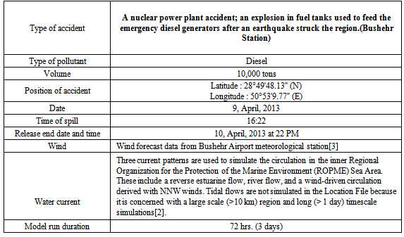
b) GNOME (General NOAA Oil Modeling Environment) was developed by the Hazardous Materials Response Division (HAZMAT) of the National Oceanic and Atmospheric Administration Office of Response and Restoration (NOAA OR&R)[2]. The program was used to simulate an oil spill occurs on the Iranian coastline on the Arabian Gulf after an accident in Bushehr Nuclear Power Plant after an earthquake occurred. The following are input data:Table (3-b). GNOME input data
 |
| |
|
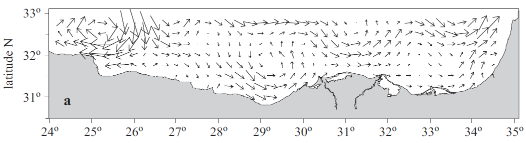 | Figure (2-a). Distribution of currents at 30 m depth off the Egyptian coast in winter |
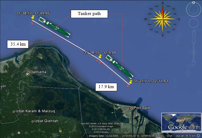 | Figure (3-a). Locations of three oil spills and the tanker path in north eastern direction of egyptian coasts |
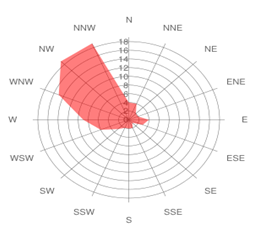 | Figure (4-b). Wind direction distribution for April, 2013 |
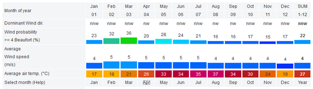 | Figure (5-b). Average wind speed and dominant wind distribution in 2013 |
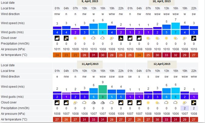 | Figure (6-b). Wind data by the meteorological Station in Bushehr Airport on 9th, 10th, 11th and 12th of April, 2013 |
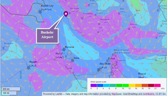 | Figure (7-b). Wind map on 9th April, 2013 for Arabian Gulf region |
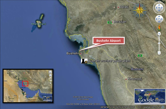 | Figure (8-b). Location of Bushehr Nuclear Power Plant in Iran |
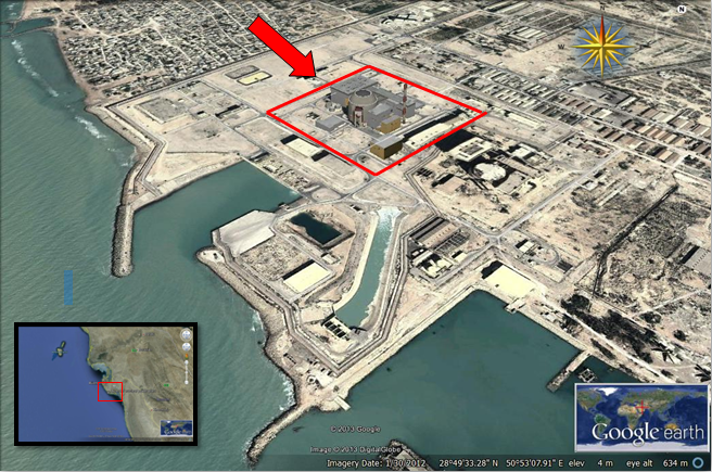 | Figure (9-b). Bushehr nuclear power plant |
3. Results and Discussions
All the above data are inputted to MEDSLIK (tanker accident on the north east coast of Egypt) and GNOME (Bushehr nuclear power plant accident on the Arabian Gulf) and the outputs are presented and summarized as follows: a) The output of MEDSLIK( tanker accident on north east coast of Egypt):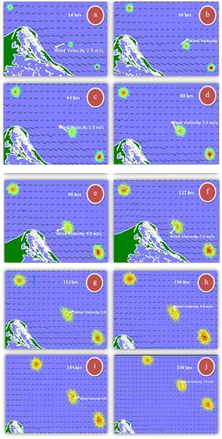 | Figure (10-a). Surface oil by MEDSLIK |
Figure (11-a) (Dispersed oil after three, five and ten days) shows that the dispersed oil propagates in the north direction away from the coastline and there's no coast impact. We used daily wind forecast data for eleven days (table (2-a)) covering the timeline of the accident simulation period (10 day), this may provide more accurate output. Figure (9-a) shows the surface oil for 10 days (240 hrs.) as wind changes as following: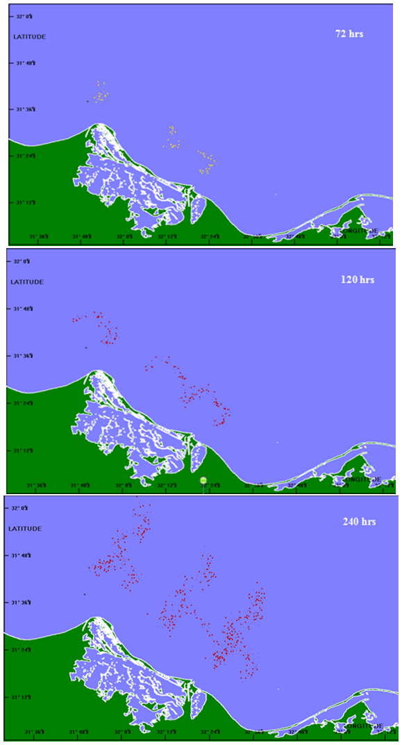 | Figure (11-a). Dispersed oil by MEDSLIK |
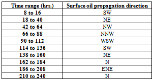
Table (4-a). Changes in the propagation direction of the surface oil for 240 hrs
 |
| |
|
Figure (12-a) oil fate parameters after 10 days (240 hrs.):a. Percentage of oil on the sea surface:ο (0 to 28 hrs.), decreases sharply.ο (28 hrs. to 240 hrs.), decreases slowly. b. Percentage of oil evaporated:ο (0 to 32 hrs.), increases.ο (32 to 240 hrs.), constant = 33.68%.c. Percentage of oil dispersed in water column:ο (0 to 240 hrs.), slightly increase to become 3.4427% after 240 hrs.d. Total percentage of oil on the coast:ο Constant = 0.0%.e. Percentage of oil on the coast but potentially releasable:ο Constant = 0/0%.Figure (13-a) oil viscosity after 10 days (240 hrs.):a. Viscosity of the oil-water mousse from the oil first released (maximum viscosity):ο (0 to 110 hrs.), increases.ο (110 to 240 hrs.), constant = 3111.71 kg/(s·m).b. Viscosity of the oil-water mousse from the oil last released (minimum viscosity):ο (0 to 114 hrs.), increases.ο (114 to 240 hrs.), constant = 3111.71 kg/(s·m).c. Oil viscosity of the oil first released (maximum viscosity):ο (0 to 26 hrs.), increases.ο (26 to 240 hrs.), constant = 100.45 kg/(s·m).d. Oil viscosity of the oil last released (minimum viscosity):ο (O to 32 hrs.), increases.ο (32 to 240 hrs.), constant = 100.45 kg/(s·m).Figure (14-a) oil density after 10 days (240 hrs.):a. Density of first oil released as percentage of density of sea water (maximum density ratio):ο (0 to 68 hrs.), increases.ο (0 to 240 hrs.), constant = 96.9%.b. Density of last oil released as percentage of density of sea water (minimum density ratio):ο (0 to 84 hrs.), increases.ο (84 to 240 hrs.), constant = 96.9%.c. Percentage of water emulsified in the oil-water mousse of first oil released (maximum water fraction):ο (0 to 68 hrs.), increases.ο (68 to 240 hrs.), constant = 72.5%.d. Percentage of water emulsified in the oil-water mousse of last oil released (minimum water fraction):ο (0 to 71 hrs.), increases.ο (71 to 240 hrs.), constant = 72.5%.Figure (15-a) slick volume after 10 days (240 hrs.):a. Volume of oil released in:ο (0 to 4 hrs.), constant = 2000 tons (first spill).ο (At 5th hrs.), step change to 3500 tons (second spill).ο (5 to 6 hrs.), constant = 3500 tonsο (At 7th hrs.), step change to 6500 tons (third spill).ο (7 to 240 hrs.), constant = 6500 tons. b. Total volume of emulsified oil in surface slick in:ο (0 to 4 hrs.), almost constant ≈ 2000 tons, but slightly increase (first spill).ο (At 5th hrs.), step change to 3500 tons (second spill).ο (5 to 6 hrs.), almost constant =3500 tons, but slightly increases.ο (At 7th hrs.), step change to 65000 tons (third spill).ο (7 to 77 hrs.), increases.ο (77 to 240 hrs.), decreases.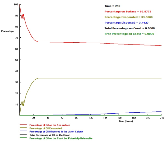 | Figure (12-a). Oil fate parameters |
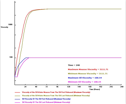 | Figure (13-a). Oil viscosity |
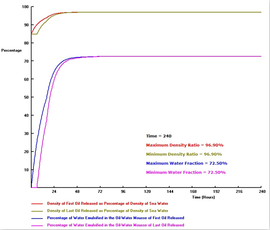 | Figure (14-a). Oil density |
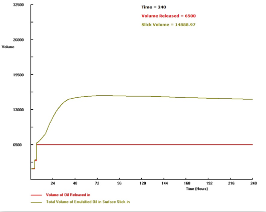 | Figure (15-a). Slick volume |
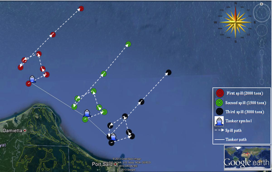 | Figure (16-a). The three spills paths for 10 days (240 hrs.) |
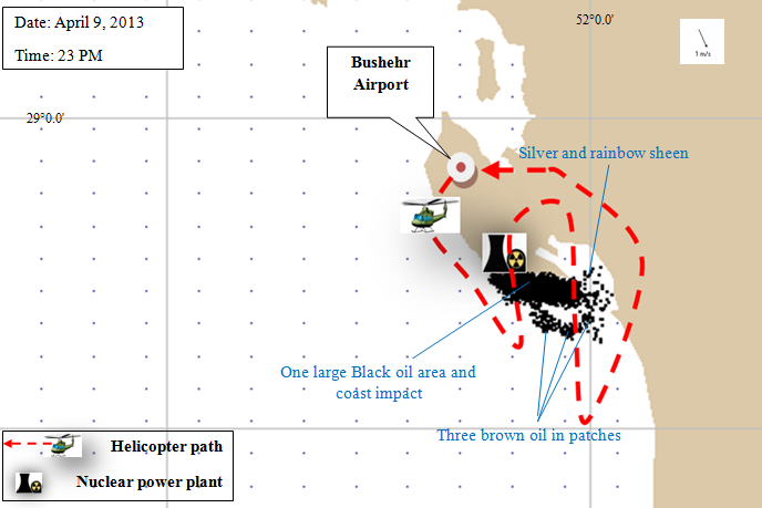
a) The output of GNOME ( Bushehr nuclear power plant accident on the Arabian Gulf:The oil spill's propagation direction during the first day is mostly south-east (figure (17-b)) and there is a large coastal impact on the coasts of Bushehr facility region. The wind directions in day 9, April, 2013 at 16 PM, 19 PM and 22 PM were W, WNW and W respectively. The directions during 10th of April are N, NW and NNE at 1AM, 4AM and 7AM respectively. It remained in WSW direction from 10 AM to 16 PM. (figure (6-b)). Later in the day, the response team is able to conduct an over flight of the spill area to visually locate slicks and sheens of oil on the water. They made aerial observations from a helicopter to spot oil on the water. One large area of black oil and three smaller areas of brown oil were spotted with silver-to-rainbow sheens trailing them to the East (figure (18-b) and figure (19-b)).The black splots (figure (17-b) and figure (19-b)) represent best guess trajectory estimate of the oil spilled from the tanker. To make this best guess, we assume that: a. The data input on the wind file accurately represent the wind directions in the timeline of the simulation for the next 3 days after the accident which is measured every 3 hours provided by the meteorological station in the Bushehr Airport (figure (3-b)). b. The data in the Location File accurately represent the current patterns during the time of the spill.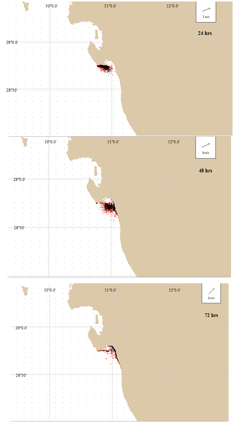 | Figure (17-b). Oil spill by GNOME after 1, 2 and 3 days |
 | Figure (18-b). Overflight map by GNOME |
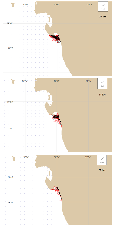 | Figure (19-b). Oil spill by GNOME after 1, 2 and 3 days after conducting an overflight |
The red splots (figure (17-b) and figure (19-b)) represent the model’s larger minimum regret trajectory estimate for the same spill. To predict this trajectory, the model accounts for uncertainty in the wind and current information that we entered. As a very rough rule of thumb—assuming a “typical” degree of uncertainty in the wind and current information, we use in modeling a spill scenario the chance that the spilled oil will remain within the area covered by the red splots is on the order of 90%. It is impossible to assign a more precise probability, because little is yet known about uncertainties in wind and current forecasts.The assumed accident scenario as follows: Immediately after the earthquake, the Bushehr reactors shut down automatically and emergency generators came online to power electronics and coolant systems. However, the earthquake had caused deformations in the earth's crust in Bushehr station region which caused seawater to flood the low-laying rooms in which the emergency generators were housed. The flooded generators failed, cutting power to the critical pumps that must continuously circulate coolant water through a nuclear reactor for several days in order to keep it from melting down after being shut down. As the pumps stopped, the reactors overheated due to the normal high radioactive decay heat produced in the first few minutes after nuclear reactor shutdown. In the high heat and pressure of the reactors, a reaction between the nuclear fuel metal cladding, and the water surrounding them, produced explosive hydrogen gas. The pool overheated, sparking fires in the building over the next hours. These massive explosions and fires reached the diesel tanks used to feed the emergency diesel generators which causes a huge leakage of oil to the sea water. About 10,000 tons of diesel was released to the sea, which caused a large oil spill in the Arabian Gulf.On April 9, 2013,anearthquake struck the Iranian province of Bushehr, near the city of Khvormuj and the towns of Kaki and Shonbeh. Seismologists said the quake struck at 16:22 (11:52 GMT) at a depth of 10 km (6.2 miles) near the town of Kaki, south of Bushehr - a Gulf port city that is home to Iran's first and only nuclear power plant (figure (20-b)). | Figure (20-b). Epicenter of the earthquake and the seismic activity fault line |
After about 2 days (48 hrs) there is coast impact on the coasts of Delvar (fig.(17-b) and fig.(19-b)) which is a city and the capital of Delvar District, in Tangestan County, Bushehr Province, Iran. Delvar is located near the coast. At the 2006 census, its population was 3,201, in 723 families. The oil spill also starts to propagate in the northern direction of Delvar (figure (21-b)) causing coast impact.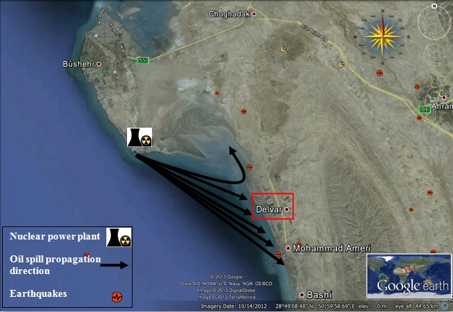 | Figure (21-b). Coast impact on Delvar city shoreline after about 2 days (48 hrs) |
4. Conclusions
1. Accidental and illegal marine pollution in the Mediterranean Sea and the Arabian Gulf constitutes a major threat to the marine environment. Previous incidents in the Mediterranean Sea and the Arabian Gulf have resulted in environmental and economic damages to fisheries, to the tourist industry and to coastal marine ecosystems.2. To prevent the major impact of accidental oil spills, local and regional preparedness and response plans recommend the use of computer-aided support systems based on operational oceanography and real-time ocean forecasts and real-time ocean forecasts coupled with satellites images and oil-spill models.3. Knowing the trajectory of the spill gives decision-makers critical guidance in deciding how best to protect resources and direct cleanup. However, it is often very difficult to predict accurately the movement and behavior of an oil spill. This is due, in part, to the interaction of many different physical processes about which information is often incomplete at the start of a response.4. The modeler must thus continuously update pre-dictions with new data and explore the consequences and likelihood of other possible trajectories, a procedure called “trajectory analysis.” The end product of trajectory analysis is often a map showing the forecast and probable uncertainty bounds of the slick movement.5. Forecasting the movement of an oil spill is often hampered by insufficient input data, particularly in the first few hours of the release. Detailed spill data (location, volume lost, product type) are often sketchy and environmental data (wind and current observations and forecasts) are often sparse or unavailable. Nonetheless, the modeler must examine the data and attempt to understand the physics and chemistry that will likely affect the oil movement and fate of the particular spill.6. As the spill unfolds, the forecast of oil movement and fate improves because the quality and quantity of the on-scene observational data improves (while initial spill data becomes relatively less important).7. Trajectory analysis should include not only the “best guess” of the oil movement and fate but also some representation of the uncertainty in the spill and environmental data used to make the forecast. The uncertainty in a trajectory forecast depends on the length and time-scale of the spill.
5. Appendix
5.1. Advection and Diffusion of the Slick
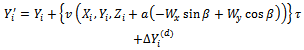
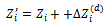
It is assumed that the surface oil is transported at a speed that is a certain fraction α of the wind speed and at a certain angle β to the right of the wind direction.In MEDSLIK, the oil spill is modeled using a Monte Carlo method. The pollutant is divided into a large number of Lagrangian parcels of equal size. At each time step, each parcel is given a convective and a diffusive displacement as follows. Let (Xi, Yi, Zi ) be the position of the ith parcel at the beginning of a particular step, Z being measured vertically upwards from the bottom. Then at the end of the time step of length τ the parcel is displaced to the point.Where u(x, y, z) and v(x, y, z) are the water velocity components in the x and y directions,Wx and Wy the components of wind velocity and 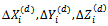 are the diffusiveDisplacements in the three directions. The vertical velocity w is not included in the model since it is generally very small.
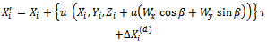 | (1) |
 | (2) |
 | (3) |
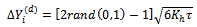
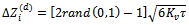
The diffusive displacements are given by: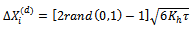 | (4) |
 | (5) |
 | (6) |
Where Kh and Kv are the horizontal and vertical diffusivities and rand (0, 1) is a uniform random number lying between 0 and 1.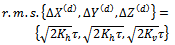 | (7) |
Kh and Kv are the horizontal and vertical diffusion coefficients. Probability of washing back on each time step τ is given by: 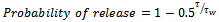 Tw is the half-life for oil to remain on the beach before washing off again. The random number generator is called and the parcel is released back into the water if Rand (0, 1) < Probability of releaseTw is assigned to each coastal segment depending on the coastal type. On each time step it is assumed that the fraction of a beached parcel seeping is
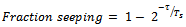 Ts is a half-life for seepage or other mode of permanent attachment.
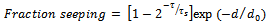 Where d is the existing density of oil on the segment (bbl /km) and d0 is a parameter. The half-life Ts for heavy oils:
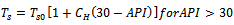 | (8) |
Where Ts0 is the default half-life
5.2. Technical Description of the Fate Models
For any sub-spill at any time step, let Vtk and Vtn be the volumes of oil remaining respectively in the thick and the thin slicks, Atk and Atnt heir two surface areas and Ttk and Ttn their thicknesses. It is assumed that the thickness Ttn of the thin slick is constant equal to 10 microns, which is a typical observed value for the final thickness of the sheen. On any time step, the two volumes are updated as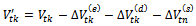 | (9) |
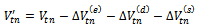 | (10) |
Where  are the volumes lost by evaporation,
  are the volumes lost by dispersion and
  is the amount flowing from the thick to the thin parts of the slick. These transfers of oil are illustrated in Figure 21.Having updated the volumes of the two parts of the slick, their areas are also updated on each step using semi-empirical spreading formulas (see below). Then the new thickness of the thick slick is computed:
 | (11) |
In the following sections, expressions based on MacKay's algorithms will be developed for all the volume and area increments.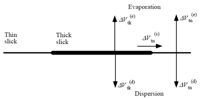 | Figure 20. Volume transfers from the thick and thin slicks |
5.2.1. Evaporation
First, for the oil in the thin slick, it is supposed that the light component evaporates immediately. The volume evaporating on each time step from the thin slick equals the total content of light component in the thin slick: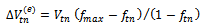 | (12) |
Where ftn is the fraction of the oil in the thin slick that has already evaporated at the beginning of the step and fmax is the initial fraction of evaporative component, which represents the maximum value that ftn can attain.For the thick slick, the increment in the fraction ftk of the oil that has evaporated is expressed as a product of the vapor pressure, Poil, and the change in an evaporative exposure, 
 | (13) |
The vapor pressure is expressed in the form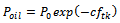 | (14) |
P0 is the initial vapor pressure and c a constant that measures the rate of decrease of vapor pressure with fraction already evaporated. The increment in exposure is expressed as a product of a mass transfer coefficient Km, the time step τ, the slick area Atk and the molar volume of the oil Vmol, divided by the gas constant R, the temperature T in °K and the initial volume of the sub-spill, V (0):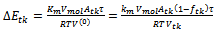 | (15) |
Where Vtk is the current volume of oil in the thick slick, equal to V (0) (1 – ftk) in the program, the various quantities are given the values Vmol= 0.0002, R = 0.000082 and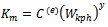 | (16) |
Where Wkph is the wind speed in kilometers per hour and C(e) and γ are coefficients with default values 0.00067 and 0.78 respectively.Then the volume loss by evaporation per time step is equal to the increment in the fraction evaporated multiplied by the original volume: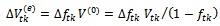 | (17) |
Although the evaporative component in the thin slick has been assumed to disappear immediately, the thin slick is fed by oil from the thick slick that has not in general fully evaporated. Thus the fraction ftn of oil in the thin slick that has evaporated must be reduced from the maximum value fmax. Equating the oil content of the thin slick before and after the inflow, we have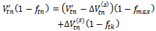 | (18) |
Where  is the updated volume, this leads to the formula
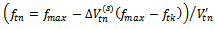 | (19) |
Having updated the volumes evaporated from the thick and thin slicks, the total fraction of the oil that has been lost by evaporation can be computed. This lost fraction is assumed to apply to all the parcels in the particular sub-spill and their fraction of light component is adjusted accordingly. Evaporation is stopped when the fraction evaporated reaches the fraction fmax of light component in the original oil. Evaporation leads to an increase in the viscosity of the oil, and the formula used for this is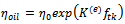 | (20) |
Where η0 is the initial viscosity and K (e) a constant that determines the increase of viscosity with evaporation (default value 4.0)
5.2.2. Emulsifications
Emulsification refers to the process by which water becomes mixed with the oil in the slick. Let fw be the fraction of water in the oil-water mousse. Then Mackay's model for the change in this fraction per time step is[16]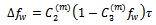 | (21) |
 constants. This model is based on assuming mousse formation is a first-order process with the water-in-oil fraction having an upper limit of
  (default value taken as 75% for light oils but decreasing with API number for heavy oils). The principal effect of emulsification is to create a mousse with greatly increased viscosity. It is supposed that the viscosity ηem of the mousse is given by
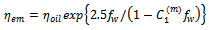 | (22) |
Where  a constant that determines the increase of viscosity with emulsification
5.2.3. Dispersion
The model of dispersion of oil into the water column is based on the work of Buist[17] and Mackay et al[16]. The process is illustrated in Figure 22. Wave action drives oil into the water, forming a cloud of droplets beneath the spill. The droplets are classified as either large droplets that rapidly rise and coalesce again with the spill, or small droplets that rise more slowly, and may be immersed long enough to diffuse into the lower layers of the water column. In the latter case they are lost from the surface spill and considered to be permanently dispersed. The criterion that distinguishes the small droplets is that their rising velocity under buoyancy forces is comparable to their diffusive velocity, while for large droplets the rising velocity is much larger.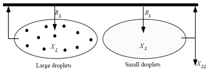 | Figure 22. The dispersion model |
Consider first the thick slick. At a given instant, let RL and RS be the downward volume fluxes of oil per unit area of the slick entering the water as large and small droplets respectively. Let the corresponding concentrations be cL and cS. If the rising velocities of the large and small droplets are vL and vS, then for a quasi-steady state we can equate the downward and upward fluxes: 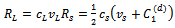 | (23) |
Where  is the (upward) diffusive velocity of the small droplets. Thus,
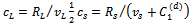 | (24) |
The total volumes of oil beneath the thick slick in the form of large and small droplets are then given by  | (25) |
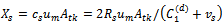 | (26) |
Where um is the vertical thickness of the droplet cloud. On each time step, a fraction of the small droplets is assumed to be lost by diffusion to the lower layers of the water column. The total volume lost on each step is taken as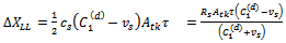 | (27) |
Where again  is the diffusive velocity of the small droplets. The total volume ofdispersed oil beneath the thick slick is then incremented according to
 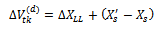 | (28) |
Where the last term represents the change in the small droplet cloud during the time step due to changing conditions (The large droplets are not regarded as dispersed since they eventually re-coalesce with the slick.) To complete this part of the model, expressions are required for the downward fluxes, RL and RS. For this, the fraction of the oil in either the thick or the thin slick that is dispersed each time step is taken as 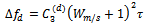 | (29) |
Where Wm/s is wind speed in m/s. For the thick slick, the fraction of this that consists of small droplets is taken as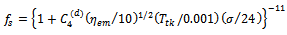 | (30) |
Where σ is the interfacial surface tension between the oil and sea water, the downward fluxes per unit area of slick per time step are then given by | (31) |
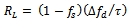 | (32) |
For the thin slick, the following simpler expression is used for the fraction of small droplets: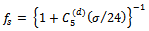 | (33) |
And it is assumed that all the small droplets below the thin slick are permanently dispersed. Thus the volume loss is given by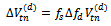 | (34) |
The total volume of oil dispersed from both thick and thin slicks, V(d) is then incremented according to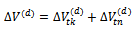 | (35) |
This gives a probability of any particular Lagrangian parcel being dispersed into the water column on the given time step equal to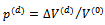 | (36) |
For each parcel the random number generator is called, and the parcel is dispersed if Dispersion is assumed to stop when the viscosity ηem of the mousse reaches a value ηmax.
5.2.4. Spreading
To complete the algorithms we need models for the changes in areas of the thick and thin slicks and the rate of flow of oil from the one into the other[18, 19]. For the thick slick, spreading consists of two parts, one a loss of area due to oil flowing from the thick to the thin slicks and a second corresponding to Fay’s gravity-viscous phase of the spreading[9]. Thus the change of area of the thick slick per time step is  | (37) |
Where  is the volume increment flowing from thick to thinslick. This volume is related to the increment in area of the thin slick:
  | (38) |
Thus, once we have a value for we can update the area,
  of the thick slick.Mackay approximates the increment in area of the thin slick by a formula similar to the Fay formula: proportional to the cube root of the area times the time step times an exponential function of the thickness of the thick slick that reflects the tendency of the slicks to stop spreading when they become very thin:
  | (39) |
Mechanical spreading is considered to occur for an initial period of 48 hours after the release of each sub-spill or until the thickness of the thick part of the slick becomes equal to that of the thin slick if this occurs first.
ACNOWLEDGEMENTS
I would like to express my sincere gratitude and appreciation to Dr. Nagwa Nassar for all of her help and valuable resources which proved to be essential while writing my paper.
References
| [1] | MEDSLIK Version 5.1.3 User's Manual, 2004, 2006, R. W. Lardner, B.A., Ph.D., Sc.D., Cambridge, UK. |
| [2] | GNOME (General NOAA Oil Modeling Environment) User's Manual, 2002, National Oceanic and Atmospheric Administration, Office of Response and Restoration, Hazardous Materials Response Division, United States of America. |
| [3] | Website for wind, waves and weather forecasts: http://www.windfinder.com. |
| [4] | M. S. Kamel, 2010 "Geostrophic current patterns off the Egyptian Mediterranean coast" study; National Institute of Oceanography and Fisheries, Kayt-Bay, Alexandria, Egypt. |
| [5] | N. Nassar, 2012 "Assessment and modeling of radiation level over North Western Coast of Egypt" Thesis; PhD; Nuclear and Radiation Engineering Department, Alexandria University, Egypt. |
| [6] | A. Amr M. Sabry, 2013" Assessment and Modeling of oil spill Dispersion on north east coast of Egypt & the Arabian Gulf" Thesis; Master; Nuclear and Radiation Engineering Department, Alexandria University, Egypt. |
 Abstract
 Reference
 Full-Text PDF
 Full-text HTML