-
Paper Information
- Next Paper
- Previous Paper
- Paper Submission
-
Journal Information
- About This Journal
- Editorial Board
- Current Issue
- Archive
- Author Guidelines
- Contact Us
American Journal of Environmental Engineering
p-ISSN: 2166-4633 e-ISSN: 2166-465X
2013; 3(5): 225-235
doi:10.5923/j.ajee.20130305.04
Water Resource Decrease Due to Land-Use Changes in the French Jura Mountains: A Combined Use of the SWAT Model and Land Cover Modeling to Evaluate the Global Trend
 Abstract
 Reference
 Full-Text PDF
 Full-text HTML
Rachid Nedjai1, Van-Tuan Nghiem2, Abelhamid Azaroual1, Laurent Touchart1, Nasredine Messaoud-Nacer3
1Institut de Géographie Alpine Université de Grenoble France (14 bis Avenue Marie Reynoard 38100 France)
2PhD Student UMR PACTE Institut de Géographie Alpine Université Joseph Fourier Grenoble France (14 bis Avenue Marie Reynoard 38100 France)
3Université de Blida Algérie
Correspondence to: Rachid Nedjai, Institut de Géographie Alpine Université de Grenoble France (14 bis Avenue Marie Reynoard 38100 France).
| Email: |  |
Copyright © 2012 Scientific & Academic Publishing. All Rights Reserved.
The main goal is to evaluate the impact of land-use changes on water resources and to predict their evolution during the next 30 years. The investigation of four landsat images (1975, 1992, 2000 and 2006) allows close detection of the landscape and shows substitution of grassland by trees, especially in higher areas. We use the LCM model with Idrisi software to predict land-use evolution and then the SWAT (hydrological model) to calculate the water flows under these new land-use conditions. The climatic conditions are kept unchanged for the predictive phase. The results show a clear decrease of the flows during the simulation period (1975-2010) which is around 15%. In fact, this observation can be related to the encroachment on landscape of landscape caused by the rural exodus recorded in France since 1970. The reduction in volume could be caused by evapo-transpiration and/or rises in infiltration generating underground circulation.
Keywords: Watershed, Flow, Land-use, Response Unit, GIS, Remote Sensing, DEM
Cite this paper: Rachid Nedjai, Van-Tuan Nghiem, Abelhamid Azaroual, Laurent Touchart, Nasredine Messaoud-Nacer, Water Resource Decrease Due to Land-Use Changes in the French Jura Mountains: A Combined Use of the SWAT Model and Land Cover Modeling to Evaluate the Global Trend, American Journal of Environmental Engineering, Vol. 3 No. 5, 2013, pp. 225-235. doi: 10.5923/j.ajee.20130305.04.
Article Outline
1. Introduction
- Most of the processes that have substantial effects on the environment and especially water systems are related to land-use change. In the French Jura Mountains, this phenomenon is highly related to the agricultural activities in the area and their reduction over the last 30 years. The transition processes are therefore the results of combining several natural and anthropogenic factors. They contribute to increased erosion processes such as chemicals transfers, and surface runoff. The acquisition of geographical data can be done by using remote sensing and GIS. The data is processed by using raster GIS techniques and several models dedicated to the evaluation of changes (LCM: Land Change Modeler), and used in the hydrological model to predict its impacts. This permits the comparison of the relative evolution of land cover over four dates, calibrating the hydrological model and finally trying to make predictions for the next 20 years. In France and especially in the mountainous areas (Alps, Jura, Vosges), the land cover shows several changes and most of the mountainous areas have seen their land-use changes progressively over the past three decades. Despite this, management forecasts are often beset by risks due to the unpredictability of the effects of the various actions envisaged. Managers may be faced with a choice between inaction or putting an action in place which has no guarantee of success.Our study will be focus on the evaluation of the degrees of change by using both remote sensing and GIS techniques which lead to the production of several models. These results provide a first basis for hydrological modelling and acquisition of useful forecast data for management. This article has two objectives: firstly, to assess the degree of transformation of forest landscape and secondly, to evaluate its impact on the hydrological dynamics of the Jura lakes and in particular the Hérisson watershed. It is a prerequisite for the transposition of treatment to the larger Ain watershed, which is a major challenge for the region. This attempt at ecological and hydrological modeling is the first of its kind in this region. It represents an innovative estimation of the evolution of vegetation cover, which provides a promising alternative for the management of large watersheds under the European framework directive.In scientific terms, the paper attempts to evaluate this combination by estimating the predictive accuracy of the analysis both concerning vegetation cover and its consequences on the hydrological dynamics of the area. In this case, it is the definition of the limits of these models and the degree of freedom of their predictions, beyond which their calculations may not be considered valid.
2. Study Area
- The study area of 53 km² belongs to the wide basin of the Ain which is a sub-watershed of the Rhône watershed. The Herisson watershed is located in the Jura department (39), in the east of France, 50 km from the Swiss border. The altitude range varies from 500 m in Val lake to more than 750 m for Ilay lake (Figure 1). The basin belongs to the Jura Mountains, being distinguished by a continental climate with few oceanic influences. The average yearly precipitations (rain and snow) fluctuate around 2 m and the average temperature is around 10°C. Most of the watershed surface (60%) is covered by trees and surrounding areas are allocated to pasture, agriculture and buildings.The site under consideration is located on the second plateau of the Jura which contains three plateaus modeled by several tectonic phases of the Jurassic and Cretaceous periods. Most of these are defined by regional faults oriented N-S which form part of the Syam network. The soil types are mainly brown earth for the first 15 cm followed by brown clay for 40 cm, amounting to around 75% of the total area. Agriculture is the principle economic activity, especially milk production, forestry and timber production.
3. Methodology and Material
- To achieve our objective, several steps were necessary as shown in Figure 2. The first step focused on data production, especially landscape characterization done using remote sensing (RS) and GIS (Geographic Information System) software. The second phase was dedicated to the definition of the principle hydrological parameters (HRU), model calibration and validation. The third part was an attempt to assess the potential impact of land-use changes on the hydrological response and finally the variation of hydrological flow in several lakes. This shows that renewal times have increased, affecting most of the principle physical characteristics of the water courses.
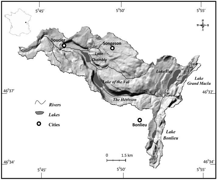 | Figure 1. Geographical location of the Herisson watershed (France) |
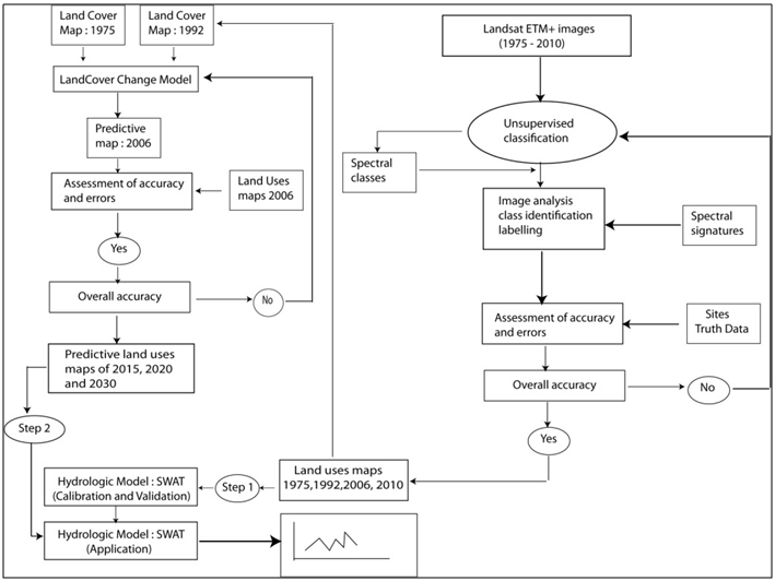 | Figure 2. Principle steps of the protocol used to evaluate the impact of land-use on hydrological flows |
3.1. Remote Sensing and Land Cover Definition
- In order to study the dynamics of land-use, maps reflecting the status of land-use at different times are required.To create these maps, four images of the study zone were used: Landsat7 ETM+ (21/09/2006 and 21/07/2000), Landsat5 TM (05/08/1992), Landsat MSS (14/07/1975). These images in the zone under consideration were taken in the same season (dry season). This limits the possibility of errors in the classification process caused by the influence of seasonal factors on the changes in vegetation. Acquired data sets were processed and examined with ENVI4.5 software. After downloading from the Global Land Cover Facility (GLCF) and importing to ENVI, the satellite data were assessed for image quality.The ETM+, TM and MSS images did not exhibit any significant radiometric noise in the entire scene. These images also confirmed geometric correction by enabling comparison of the positions of specific points on the images and on the topographical map. The results showed that the geometric correction of the images is within acceptable standard (less than 1 pixel).Before actual image classification, the spatial resolution of the images had to be synchronized. The original resolution of the MSS image was 57 x 57 meters. To compare this with the ETM+ and TM images, whose resolutions are 28.5 x 28.5 meters, the MSS image needed re-sampling. The ETM+ 2006, ETM+ 2000, TM 1992 and MSS 1975 images were classified using the Maximum Likelihood supervised classification, the most popular method used for quantitative analysis of remote sensing data (Pontius et al., 2007). This method is based on using appropriate algorithms for pixels’ classification in an image. Many algorithms are available for classification, such as the ones based on models of probability distribution (Pontius et al., 2007; Perumal et al., 2010). According to several studies (Cetin et al., 2004; Frinelle et al., 2001; Gholami et al., 2010; Akgün et al., 2004; Perumal et al., 2010), the Maximum Likelihood algorithm provided the most accurate and the most stable classification results. In addition, our experiments made during this study have again proved the above observation. The images from the seven predominant land-use types of the Herisson basin were classified in a monitored way: conifers, mixed forest, farm land, built-up areas, water and meadows. This was done by considering the spectral signatures from the training sites which were selected. Finally, the classification of images was processed. With this procedure, four maps of land-use for 1975, 1992, 2000 and 2006 were generated.The validation for the categories was performed through the observations taken in the area. The purpose was to determine the number of observations that matched the classification which was undertaken, to estimate the level of correction. The overall accuracies of the land-use maps for 2006, 2000, 1992 and 1975 were 86.50%, 85.67%, 88.19% and 85.92% respectively, and the Kappa indices for each map were 0.83, 0.82, 0.83, and 0.84.
3.2. Land-use Prediction and Hydrological Modeling
- The second part of the study involves the production of a scenario of land-use change and the generation of predictive maps for the next 30 years. For processing and prediction, the LCM developed by the Clark Labs (Idrisi) was used to analyse land-use (Eastman J.R., 2001; Eastman J.R., 2003; Eastman J.R., 2006). Several studies had shown the effectiveness and accuracy of these methods based on the Markov Chain and the use of regression models (Neuronal and logit models) (Eastman J.R., 2006; Aguejdad et al., 2008) to improve the predictive results and help managers (Oñate-Valdivieso., 2010). The method used for analyzing the changes is that proposed by Pontius et al., 2004. This method allows the determination of persistence, gain or the loss, and substitution between categories. Three pairs of maps (1975, 1992), (1992, 2000), and (2000, 2006) were used to generate the predictive maps. This phase helped us first to identify potential relationships between land-cover changes and potential explicative variables, and then to validate the predictive model by comparing these results with the maps from 2000 and 2006. A cross tabulation was automatically generated, and the changes that occurred during the three analyses of (1975, 1992), (1992, 2000) and (2000, 2006) were determined respectively. Only the comparison between 1992 and 2000 was used in this study and considered as a sub-model of transition. Two steps distinguish this part of the study: 1) the focus on the selection of the explanatory variables, and 2) the creation of predictive maps for 2015, 2020 and 2030. The calibration of the model was made by comparing the predictive maps for 2000 and 2006 with observed maps from RS processing for the same dates. The statistical processing was performed by the use of XLStat software and the determination of the Cramer V coefficient, which allowed the variables with high explicative potential to be evaluated. Only Cramer coefficients higher than 0.15 were considered and included in the transition model (Eastman J.R., 2006; Oñate-Valdivieso et al, 2010). The matrix of the Cramer coefficients was obtained by comparing the variables. Nine variables were considered including: topography (DEM), distance from built-up areas, distance from water, distance from roads, distance from coniferous forest, distance from mixed forest in 1992, and distance from farmland.The spatially distributed hydrological models are used by several studies for their ability to represent basin dynamics. So, to assess the land-use impacts on the water flow in the Herisson basin, the use of this kind of model seems appropriate to prediction of environmental change especially within the hydrological system (Rafael Hernandez Guzman et al., 2009).For the hydrological modeling, the SWAT (Soil Water Assessment Tools) model was selected and used to perform the simulation and to evaluate the flow fluctuations of lakes, especially of Ilay, the largest lake. Considering basin and sub-basin scales based on the natural limit (boundary) is one of the most reliable hydrological approaches to appreciate water movement. This method gives all informations necessary for understanding the heterogeneity of watersheds, especially the processes. The extraction of topographical features (drainage network, watershed delineation and slope) is described in the literature (O'Callaghan et al., 1985; Jenson et al., 1985; Jenson et al., 1987; Jenson et al., 1988). Three steps are necessary:− Watershed delineation: GTOPO30 Dem (with 25 m resolution ) and Digitized streams are used; the outlet corresponds to the measurement point of the DREAL. This step is achieved by the use of RS and GIS. Some errors can be made by the aggregation of areas which causes a drastic reduction in accuracy due to the loss of information. The best choice is to define a small area that is relatively homogenous (HRU) in terms of soil, land use, topography, slope, ...− Soil maps are issued from the combination of land-use/land-cover maps, the geological map, and the field test for soil. These land-use and soil maps are then used to perform the HRU units (Rafael Hernandez Guzman et al., 2009; Arnold et al., 1998; Arnold et al., 2005).− Climate data: all data are collected from the personal weather station, belonging to the research team, and from Météo France. The period covered is 1975-2010.The calibration was made with observed data concerning measured, locally produced parameters. Indeed, the simulated data is compared with both the DIREN measures of flow performed during the period 1975-1980 and our measurements of water level obtained by the installation of instruments (Mini Troll 300) in the four lakes.
|
4. Results and Discussion
4.1. Processing and Analysis of the Remote Sensing Results
4.2. Definition of the Explicative Variables and Analysis of Land-use Changes
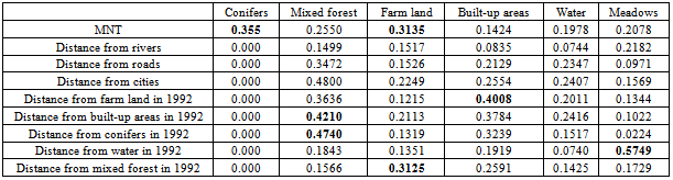
- Precipitation is one of the variables commonly used in the literature (Oñate-Valdivieso., 2010). In this case, based on the low ranges of altitude, the spatial variability of this parameter is relatively small and cannot be used as an explicative variable. This is also applies to the slope of the topographical structure of the site (plateau) and the reduced values recorded. It can be seen from the analysis of Table 1 that:− The coefficient of the distance from rivers is much smaller than that of the other variables, and has a much reduced correlation with the other six categories, especially with coniferous woodland, water and built-up areas.− The correlation between the six categories and topography is very limited even if the association between conifers and agriculture can be considered as acceptable with values of around 0.35. Distance from roads and from cities presents acceptable correlations with mixed forests, respectively (0.34) and (0.48).− The highest correlation is recorded predominantly for coniferous woodland and topography, and for grassland and topography. This observation has been seen in other regions in France (Lake Val) and in other countries.The homogeneity of soils and the small surface area of the watershed make it impossible to use these qualitative variables.
4.3. Modeling the Land-use Changes and Validation of the Model
- To evaluate the changes, the probability of the occurrence of each transition was calculated by using two models: the MLP (Neuronal networks) (Eastman J.R., 2006; Rocha et al., 2007; Canziani et al., 2008) and Logistic regression (Judex., 2006; Zeng et al., 2008; Lacono et al., 2009). These models are based on the explicative variables selected above and the observed changes evaluated from the comparison of the different maps generated by RS (Eastman J.R., 2006). In this first step, a predictive map for 2000 is created by using the coverage of 1975 and 1992, and the transition probability is initially calculated using the Markov Chains (Stewart W.J., 1994; Weng Q., 2001; Eastman J.R., 2003; Mubea et al., 2010; Yang et al., 2011). To complete and to verify the probability of the transition, two other maps for 2000, 2006 were generated with the same probabilities used previously (Pontius et al., 2004).These predictive maps are then compared to the reference map, made by RS in order to calculate the errors. The error values, calculated by comparing maps observed in 2000 and 2006, considered as a reference, with the maps obtained by the application of MLP and Logistic regression, range between 10 and 15%. With these values, the model can be considered acceptable and stable. Matrix confusion was used to compare the reference with the predictive maps (Table 2). The Kappa index calculated from the reference and predictive maps, and a comparison of the number of pixels which had been correctly assigned and the total pixels of the image, showed the reliability of the classification (Pontius et al., 2004; Falahatkar et al., 2011) .These two maps (1992, 2000) were used to evaluate the areas of loss or gain for each category and to show the tendencies on the plateau during the period under consideration. This step allowed predictive maps to be created by using the MOLA method and by considering all observed changes (transition). Based on this adjustment, three land-use maps were generated for 2015, 2020 and 2030, respectively. This phase was used to appreciate the pertinence of the model under these new conditions. Two of the three generated maps were then used to simulate the evolution of the flows and volumes of water in the five lakes.
4.4. Transition Sub-models
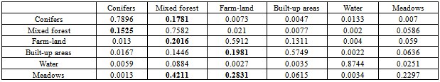
- In general, sub-models of transition include explicative variables with values higher than Cramer’s V (20). The variables which contribute to improving the correlation between transition and explicative variables are used. Table 2, presented below, shows the results from sub-models of transition, the variables integrated into these sub-models and the coefficients of logistic regression. This list is completed by the coefficient that affects explicative variables in the logistic regression equation and the degree of correlation between the explicative variables and the transition (ROC) (Pontius et al., 2001). The correlation always exceeds 89%. All values are around zero, and this shows that the relationships between variables are highly influenced by the small size of the watershed, the modest changes in topography and the similarity of the climate. Despite the low variability of the topography, this is positively related to coniferous or mixed forest, which confirms that the forest globally covers the higher parts of the watershed. The transition of land-use from agriculture to coniferous or to mixed forest shows a positive correlation and confirms that most of the agricultural areas located in the higher zones of the watershed have been progressively replaced by trees (mixed forest) and the enclosure of the landscape over recent years. In general, the pasture (grassland) has a positive correlation with the distance from settlements and roads. This is due to the fact that farmland is often close to built-up areas and in the downstream areas of the watershed. On the contrary, the transition from forest to grassland is positively correlated with the distance from cities and roads. Therefore, the accessibility to these areas promotes their continued use.The distance from farmland in 1992 is inversely related to the transition from grassland to agriculture and from mixed forest to coniferous woodland (≈ 0.15). On the other hand, the correlation is positive between the distance from settlements and the transition from agriculture to buildings. This confirms the extension of settlements in recent years, especially in the downstream areas of the watershed, particularly those near to the Champagnole settlement. In the validation phase, the use of MLP (Multilayer Perceptions Neuronal Networks) results in a low level of RMSE error. The accuracy in modeling transitions is around 76% in all cases.The probability of transitions for each category of land-use is shown in Table 2. A high likelihood of transitions is observed between meadows and mixed forest (0.42). This shows that there is slowing down of farming activities in the watershed and the progressive landscape closure. This phenomenon is followed by the transition from the agricultural areas to grassland which confirms the continuity of the process discussed above. Several other transitions are seen inside the forested areas such as the substitution of coniferous forest for mixed woodland in the middle of the watershed. The coefficient, around 0.15, explains the predominance of timber production and a reduction in agricultural activity. This observation is recorded regionally throughout most of the Alps and Jura areas, as has been mentioned by many authors.
4.5. Validation of Land-use Change Models
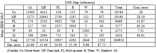
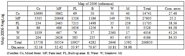
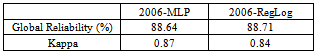
- The model is validated by comparing the maps built by both the logistic regression and neural network methods with the map extracted from the 2006 image (Pontius et al., 2004; Pontius et al., 2005). The results are included in Figure 3. The first observation resulting from a visual comparison of the predictive and reference maps obtained from the Landsat ETM+ image of 2006 shows that with the logistic regression method, similitude is very high downstream of the watershed and very low in upstream areas. Inversely, the difference is high within the map built with the MLP method. The principle difference is registered on the built-up areas located close to older settlements and derives from the transition of the agricultural areas.We observe, after comparison with field surveys, an over-estimation of the areas covered by buildings in the higher zones and a reduction of the areas covered by grassland or by the agricultural use.The confusion matrix between the maps which are predicted with Logistic regression and reference extracted from the 2006 Landsat ETM+ image is presented below. The first observation is the large number of pixels which show a correspondence between the thematic types of the two maps. On the contrary, several pixels (3505), observed as coniferous in the 2006 image, were classified as Mixed Forest in the predictive map (RegLog). On the other hand, around 1000 pixels belong to the grassland type in RegLog map while they are classified as coniferous in 2006 image. The global reliability calculated from the confusion matrix is shown in Table 3 and Table 4.
|
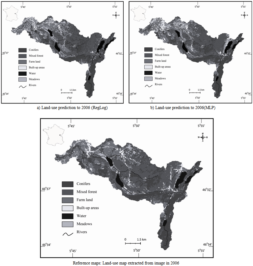 | Figure 3. Comparison between the reference map and maps predicted with (a) Logistic Regression and (b) Neural Network MLP |
|
|
|
5. The Impact of Predicted Land-use Changes on Water Storage in the Ilay Lake
- The principle aim of this step is to evaluate the impact of land-use change on the water flow and more widely the potential decrease of water volume over the next 30 years. The predictive land-use maps obtained using the LCM model allow the potential impact on water quantities to be evaluated. The simulations were made in two steps:− The first step focuses on the use of current parameters (climate and land-use) to simulate the water flow within the watershed. The period considered in this step goes from 1975 to 2010. The comparison of the daily simulated data with the observed data and the calculation of the Nash coefficient (0.90) confirms the calibration of the model. The result shows a relative decrease of water flow, particularly during the period between 1987 and 1991, known as a dry period. The latter period is confirmed by many studies, see for example the case of the river Rhône (DIREN Rhône-Alpes., 2001)− The use of predicted land-use for the same period shows a relative decrease in the volumes estimated by 10-15 % (Figure 5). The daily volumes can be considered stable and no trend is registered.The calculation of the year-on-year variability in volumes shows a clear trend during this period and confirms the decrease and the impact of land-use change as illustrated in figure 6.
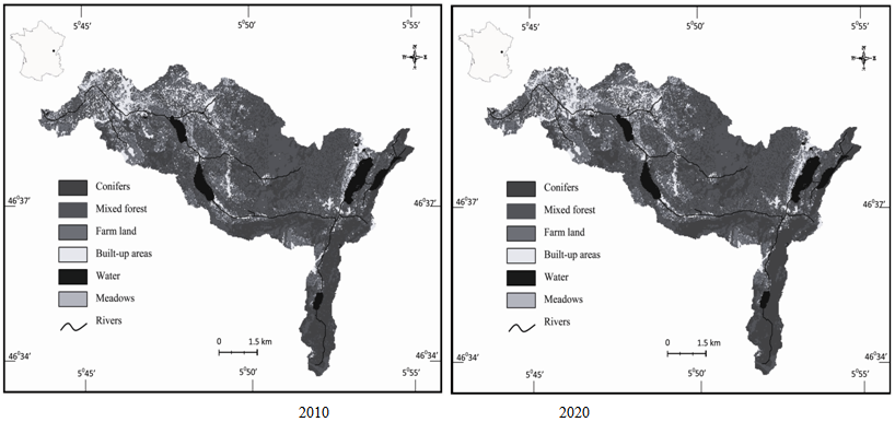 | Figure 4. Predictive maps for 2010 and 2020 built for Herisson basin |
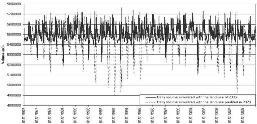 | Figure 5. Water volume comparison between land-use in 2006 and 2020 |
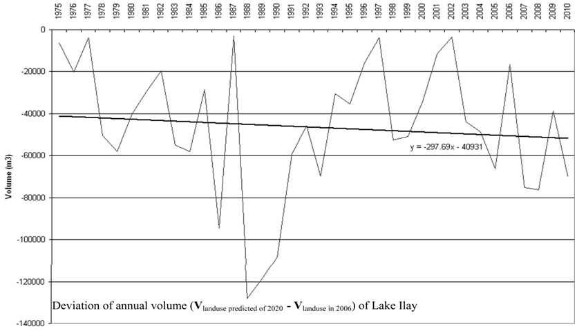 | Figure 6. Annual decrease of water flow for Ilay Lake |
6. Conclusions
- The question of the impact of land-use changes on limnic systems, and more widely on whole ecosystems, has been of particular importance over the past thirty years, marked by signs of global warming and the mass exodus of farmers.The Jura Mountains and especially the lakes translate the modification experienced by the evolution of the land-use during the last 30 years (from the middle of the 70s). This phenomenon is principally related to the progressive closure of the landscape. These spaces have been replaced by trees, coniferous and mixed forest. There are changes in most of the categories especially that related to mixed forests with an increase in their surface area, followed by a lesser increase in that of coniferous woodland. The agricultural surface area has been drastically reduced, benefitting pasture and urban areas which are common in the Jura and throughout rural regions in France. The exodus of farmers recorded over the last 30 years is followed by the closure of wide areas especially in the higher parts of the watershed. The output flow is dependent principally on land-use change and secondarily on extraction for domestic consumption. However, this second factor is relatively unimportant. The main results show a clear change in land-use which is accompanied by a trend towards lower levels of lakes, hence a decrease in water volume of the order of 15%. This deficit may be due to the combined effect of evapo-transpiration and the interception of precipitation by forests. For this, the reintroduction of agricultural activities cannot be the only solution because of political and economic policy guidelines in France. However, it is important to perform regular maintenance in these areas in order to minimize the process of natural reforestation.
ACKNOWLEDGEMENTS
- The authors would like to thank the local government body for giving us all the necessary authorisations and Mr Stéphane Forne for his collaboration.