1. Introduction

In recent years the Climate Change Problem raised the discussion of limiting and reducing greenhouse gas emissions caused from the burning of fossil fuels, by substitution of these limited resources with renewable and clean energy sources. One promising energy supplier among others is, as sometimes announced, “harnessing the wind”. Although, eolic energy generator technology has left its childhood already some time ago, there are still challenges to be faced in order to restrict or remove certain uncertainties related to this type of electric energy production. The incorporation of eolic energy into the total energy demand still suffers from the fact that supply of wind power depends directly on the wind conditions so that the energy to be injected into the electrical network will be strongly governed by the wind variations but not by the energy demand. In fact, this is the reason why wind energy is said to be unreliable, because of its natural fluctuations. In order to mitigate these difficulties it is of interest to study the wind conditions and its inherent variations on a short term (daily) basis, and a seasonal or long term basis, and turn more predictable the availability of eolic power for a specific site. This knowledge could give support to the management of future wind-park clusters through an additional tool that shall help to minimize or even control the aforementioned variations using probabi-lity based energy distribution plans.

One of the issues addressed in the present article is related to the choice of the site for a possible installation of a wind park considering meteorological aspects as well as possible scenarios simulations and their related experimental validation. One of the possible evaluations of a site candidate may be performed using tracer experiments in order to analyse the wind conditions in the planetary boundary layer, which is typically the layer where eolic turbines are placed. Since this kind of experiments are performed only in a limited set of positions the entire wind velocity field may be reconstructed only by the use of reliable models. However, these models have to be tuned using specific meteorological parameters and conditions in the considered region and shall be subject to the local orography. Furthermore, case studies by model simulations maybe used to establish limits for the generator density using studies with data from already working wind-parks together with model simulations. To this end, existing eolic farms may be used in order to study the influence of generators on changes in the boundary layer wind profile. Such a time sequence analysis may well be performed using tracer experiments, where from the observations one may reconstruct the full space-time wind field by models. This may help to optimise the arrangement of a wind generator cluster taking into account the turbulent structure of the wind field that may in principle be modelled with and without the presence of wind generators. Recent research[11, 38] pointed out the relevance of the mutual wind turbine interaction as well as the impact of the wind flow perturbation by turbines on the atmospheric boundary layer in wind farms with extensions beyond the length scale defined by the boundary layer height. In their work the authors quantified the vertical transport kinetic energy and momentum across the boundary layer, which was found to be of the same order of magnitude as the power extracted by the forces that modelled the wind turbines. This finding was directly associated to atmospheric boundary layer turbulence, which is the focus of the present article.

In references[11, 38] a model for the wind energy generators was used to simulate effects on the boundary layer. The present discussion complements the previous works in the sense that one may reconstruct the wind profile with its turbulent properties for the different stability regimes in the planetary boundary layer using data from observations instead of simulating them and tuning the model as to agree reasonably well with the experimental findings. More specifically, the measured average wind velocity field is used (see reference[27]) together with probability density functions, that depend on the stability regime in consideration, and the turbulent contribution is then determined from the nonlinear stochastic Langevin equation. This procedure may be used for analysing potential wind energy park sites or already existing ones. The choice for a Lagrangian model in comparison to an Eulerian approach resides in the fact that the latter yields average values only, whereas Lagrangian models capture the stochastic characteristics of the turbulent wind field by virtue of the employed probability density functions. The mapping of turbulent wind fields instead of mean fields is essential for opening pathways that help increasing the predictability of the wind profile in all stability regimes along the 24 hour cycle, and especially during stability changes. During changes of stability and in the unstable regime, energy of the mean field is transferred to the turbulent field that affects the gain in energy conversion by wind turbines.

In the further we show how the Langevin model is solved analytically using the decomposition method which then may provide short, intermediate and long term (normalized) behaviour and permit to assess the probability of occurrence of higher or lower turbulence levels and additionally serve as a supplement for designing the afore mentioned energy response plans. Note, that natural turbulence is one of the reasons for a decrease of the efficiency of the turbines from its nominal value, and the square ratio of the turbulent velocity to the mean velocity represents a crude measure for that effect. A further aspect worth mentioning is that the average eddy size is roughly of the order of magnitude of the rotor.

The stochastic character of turbulence is implemented using the appropriate Gaussian, bi-Gaussian and Gram - Chalier probability distribution for the different stabilities. Exactness of the solution is manifest in stable convergence, which we control by a Lyapunov theory inspired criterion. The most adequate probability distribution for the wind scenario of interest is indicated by a novel statistical validation index, which from comparison to experimental data selects the most significant model. Comparison to the Copenhagen and to other deterministic approaches shows the advantage of the present analytical approach even for considerably rugged land relieves.

Our article is organised as follows. In section 2 we report on the state of the art of stochastic wind profile modelling, and show how a closed form solution may be obtained by Adomian’s decomposition method. In 3, we present the numerical results for three probability density functions and in section 4 we come to our conclusions.

2. Stochastic Wind Profile Modelling

Atmospheric turbulence and tracer dispersion in the planetary boundary layer is a stochastic process and thus obeys a stochastic law which may be expressed as a set of stochastic differential equations. For a time dependent regime considered in the present work, we assume that the associated Langevin equation adequately describes atmospheric turbulence and dispersion processes, which we test by comparison to other methods in order to pin down computational errors and finally analyse for model adequacy. We are aware of the fact that up to date there do exist a variety of models and approaches to the problem, either based on numerical schemes, stochastic simulations or (semi-) analytical approaches and indicate in the further a selection of models. Numerical approaches may be found in the works of Tangerman[45], Brebbia[8], Chock et al.[17], Sharan et al.[41] and Huebner et al.[31]. There are various models that have been used effectively in the past to describe tracer dispersion[48],[42],[6],[5], and many of them make use of analytical approaches[35, 42, 43]. One also finds semi-analytical methods, where we mention the works of Parlange[39], Dike[20], Henry et al.[29], Grisogono and Oerlemans[25], Metha and Yadav[37], Carvalho et al.[13] and Carvalho and Vilhena[12].

Upon developing a model one typically faces various problems. First one has to identify a differential equation that shall represent a model or a physical law. Once the law/model is accepted as the fundamental equation one challenges the task of solving the equation in many cases approximately and analyse the error of approximation and numerical errors in order to validate its prediction against experimental data. Experimental data of a stochastic process typically spread around average values, i.e. are distributed according to probability distributions. Hence, the model shall within certain limits reproduce the experimental findings. Since the fundamental equation is already a simplification deviations may occur which in general have their origin in a model error superimposed by numerical or approximation based errors. In case of a genuine convergence criterion one may pin down the error analysis essentially to a model validation. Since in general convergence is handled by heuristic convergence criteria, a model validation is not that obvious. Thus we show with the present discussion, that our semi-analytical approach does not only yield an acceptable solution to the Langevin equation but predicts tracer concentrations closer to observed values than predictions from other models values with is also manifest in the statistical analysis.

Simulation of tracer dispersion in the Planetary Boundary Layer (PBL) through a Lagrangian particle model by the use of the Langevin equation and its diffusion equation limit (random displacement equation) usually has been solved by the method of Ito calculus[24, 40]. More recently one of the authors developed the Iterative Langevin Solution (ILS) method, which solves the Langevin equation in a semi-analytical manner by the method of successive approximations, known as Picard’s iterative method. The method is principally characterised by the following steps: Application of Picard’s procedure on the Langevin equation, to be more specific, integration, linearisation of the stochastic non-linear term and iterative solution of the resultant equation, which permits to evaluate an analytical expression for the velocity. Details of this approach may be found elsewhere[13, 14, 12, 44, 15, 16].

An alternative analytical method for solving linear and non-linear differential equations was developed by Adomian[1], known as the decomposition method. The decomposition procedure permits to cast the solution into a convergent series by using the necessary number of recursions for both linear and non-linear deterministic and stochastic equations. The advantage of this method is that it provides a direct scheme for solving the problem without the need for linearisation or transformations. There exists a vast literature about applications of this method to a broad class of physical problems and we cite the works we considered relevant for the further discussion[1, 2, 3, 22, 34, 32, 19, 21]. Thus the present work extends the list of methods that solve the Langevin equation assuming Gaussian, bi-Gaussian and Gram-Chalier turbulence condition by Adomian’s approach. The variety of methods, such as the numerical solution of the Langevin equation (integrated according to the Ito calculus), analytical solution of the Langevin equation (derivation of Uhlenbeck and Ornstein[47]), Iterative Langevin Solution (ILS) and solution by decomposition (ADM)[26].

2.1. The Decomposition Method for a Stochastic Process

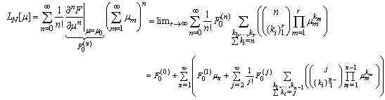
A time dependent stochastic process µ is typically characterized by its time evolution, which depends on stochastic contributions, such as expectation values (E_n) of mean field character (E₀) and higher moments (here E₂), respectively. In our case we consider the Langevin equation to describe turbulence.

(1)

Here is a stochastic measure for random motion and E₀ represents a drift like term, whereas E₂ is a measure for diffusion intensity, which satisfy the usual Lipschitz continuity condition in order to ensure the existence of a unique strong solution. In case of a Wiener process µ(t) is Markovian, but in our case we presume that the process is an Ito process, i.e. it depends on the present and previous values, hence the integral form of mean field and fluctuation contributions. Note, that the integral form will be used further down in order to set-up the solution following Adomian’s prescription, which we resume in the following.

One may rewrite the stochastic equation from above (1) as a differential equation, upon using the limit τ→ 0 and separating all terms depending on the process µ including the differential operator (LHS of equation(2)) from the noise generating term G(t) (the stochastic contribution, last term in eq. (1)).

(2)

According to Adomian, one splits the linear operator, that includes the derivatives L_L with known inversion from the non-linear terms L_N. Further we write µ(t) as a sum of a convergent sequence µ_i(t), still to be specified, and the nonlinear term is cast into a sum of so called Adomian functional polynomials[1].

(3)

For the nonlinear part we use a normal convergent operator expansion

(4)

and rewrite the non-linear term as

(5)

where we introduced the shorthand notations for the derivative terms F₀⁽ⁿ⁾ the polynomial coefficients. Introducing these terms into the original differential equation permits to identify corresponding terms, that give rise to the iterative scheme in the spirit of Adomian as shown next.

(6)

There are many possibilities to setup an iterative scheme which upon truncation to n terms in A_n and n + 1 terms in µ_n yields an approximate solution in analytical form. Instead of solving the original Langevin equation we cast the problem into a set of simpler equations which may be solved because the integral operator L_L^-1 is known.

(7)

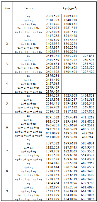
The way we have setup the iterative scheme defines the seed µ₀(t) by the stochastic contribution as source term, whereas the remaining iterators are simply given by the Adomian functional polynomials as source terms of the equations to be solved. Note that in order to evaluate the i-th recursion step µ_i the µ_j with j < i are known from the previous iteration steps. Moreover, the functional expansion of the non-linear term around the function µ₀ shows how the stochastic term effectively enters in the remaining terms µ_i with i > 0 from the non-linearity.

2.2. A Convergent Closed Form Solution

The iteration defines a convergent series towards µ for all t in a certain domain, thus the solution is manifest exact. Since this scheme defines an explicit analytical expressions for the µ_i and A_i, respectively, one arrives at a procedure which permits to solve the differential equation without linearisation in closed form. The procedure has been applied to a variety of nonlinear problems but an analytical procedure for testing convergence to the best of our knowledge has not been presented in literature, only numerical schemes may be found, see for instance refs.[32] and[4].

In general convergence is not guaranteed by the decomposition method, so that the solution shall be tested by a convenient criterion. Since standard convergence criteria do not apply for the present case due to the non-linearity and stochastic character, we present a method which is based on the reasoning of Lyapunov[9]. While Lyapunov introduced this conception in order to test the influence of variations of the initial condition on the solution, we use a similar procedure to test the stability of convergence while starting from an approximate (initial) solution µ0 (the seed of the iteration scheme).

Let us denote the maximum deviation of the correct from the approximate solution , where || ∙|| signifies the maximum norm. Then convergence occurs if there exists an n₀ such that the sign of λ is negative for all n ≥ n₀.

(8)

In the further we apply the decomposition method as presented in general form above to the problem of tracer dispersion for three different turbulence probability density functions, i.e. Gaussian, bi-Gaussian and Gram-Chalier, respectively. The analysis of convergence is applied to all cases that shows that for n₀ = 4 the approach is convergent with an error less than 1%.

3. The Langevin Equation for Stochastic Turbulence

The stochastic equation (1) may be interpreted in terms of the Langevin equation, where µ represents the turbulent velocity vector with components u_i. In the Langevin equation[40] the time evolution of the turbulent velocity is driven by a dissipative term and a second term which may be understood as the gradient of a potential that depends on the fluctuations of the turbulent velocity and represents a mean field interaction of the tracer with the environment it is immersed. The last term represents the stochastic contribution due to a continuous series of particle collisions. All paragraphs must be indented.

(9)

Here u_i with i = 1, 2, 3 is a Cartesian component of the turbulent velocity, which is related to the infinitesimal displacement and the wind velocity U_i by dx_i =(U_i + u_i)dt. The coefficients α_i, β_i, γ_i of eq. (9) depend on the employed probability density function. Here C₀ is the Kolmogorov constant, ε is the rate of turbulence kinetic energy dissipation, and ξ_i is a random increment according to a probability density function.

Upon application of the described decomposition method from above (see 2.1) on equation (9), the turbulent velocity is decomposed into a series and the non-linear contribution is taken care of by Adomian’s procedure.

(10)

where the non-linear term is .

Table 1. Meteorological parameters measured during the Copenhagen experiment. L is the Monin-Obukohv length, zi the convective boundary layer height, u* is the local friction velocity, w* is the convective velocity scale, U(10) is the wind speed in 10 m and U(115) is the wind speed in 115m and h is the PBL height

In the iterative scheme the stochastic component is absorbed in the first term u₀ of the expansion and thus propagates through all subsequent terms, whereas the nonlinear (mean field) term enters as a correction from the second term on. For any given truncation m the solution for the considered problem (9) is given in closed analytical form summing up the terms .

So far we have not defined the probability density function, that characterizes the type of turbulence which is correlated to the stability of the planetary boundary layer (PBL). In the studies of turbulent dispersion the stochastic behaviour maybe classified according to stationarity or non-stationarity, according to spatial properties as homogeneity or non-homogeneity and according to the profile of the wind distribution, as Gaussian or non-Gaussian. When employing Lagrangian models one usually considers stationary and homogeneous turbulence in horizontal sheets and non-homogeneous and either Gaussian or non-Gaussian in the vertical direction depending on the stability condition. In stable or neutral conditions the velocity distribution may be considered Gaussian, whereas during convective conditions the velocity distribution is non-Gaussian because of the skewness of the turbulent velocity distribution, which has its origin in up-and down-drafts with different intensity. In the following we present the solutions for the three afore mentioned probability density functions together with their model validation against the data from the Copenhagen experiment[26].

3.1. The Copenhagen Experiment

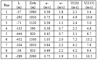
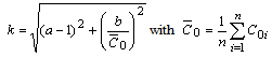
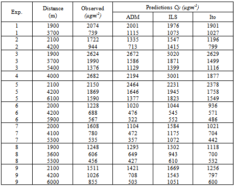
The Copenhagen tracer experiment[26] was carried out in the northern part of Copenhagen. A tracer (SF6) was released without buoyancy from a tower at a height of 115m and collected at the ground-level positions in up to three crosswind arcs of tracer sampling units. The sampling units were positioned 2km-6km from the point of release. A total of nine tracer experiment runs were performed with instability conditions as shown in table 1. The site was mainly residential with a roughness length of 0.6m. Wind speeds at 10 and 115 meters were used to calculate the coefficient for the vertical exponential wind profile, which is used to model the wind speed.

(11)

where U(10) is the wind speed in 10m and U(115) is the wind speed in 115m, respectively.

For the simulations, the turbulent flow is assumed inhomogeneous only in the vertical direction and the transport is realized by the longitudinal component of the mean wind velocity. The horizontal domain was determined according to sampler distances and the vertical domain was set equal to the observed PBL height. The time step was maintained constant and was obtained according to the value of the Lagrangian decorrelation time scale (Δt = τ_L/c), where τ_L must be the smaller value among τ_Lu, τ_Lv, τ_Lw and C is an empirical coefficient set equal to 10. In Equation (10), the product C₀ε is calculated in terms of the turbulent velocity variance σ_i² and the Lagrangian decorrelation time scale τ_Li[30, 46], which are parametrised according to a scheme developed by Degrazia et al. ([18]). These parametrisations are based on Taylor’s statistical diffusion theory and the observed spectral properties. The concentration field is determined by counting the particles in a cell or imaginary volume in the position x, y, z. The integration eq. (10) was computed by the Romberg method.

3.2. Solution for Gaussian Turbulence

In the case where a Gaussian probability density function describes best the stochastic turbulence the coefficients of the Langevin equation (9) and (10) are

(12)

In Table (2) we compare the experimental findings with the model predictions by the proposed procedure (ADM – Adomian Decomposition Method), by the Ito method[40], by the ILS method[12] and the early analytical derivation (ANA) by Uhlenbeck and Ornstein[47]. From the comparison one observes a reasonable agreement among the models and also with the experimental data. In the following table the numerical convergence of the ADM approach for a Gaussian probability density function (pdf) is indicated. The convergence analysis shows that already a few terms represent an analytical solution with spurious error only. The figures 1 show the Lyapunov exponent of the Adomian approach depending on the number of terms for the 9 experimental runs. Note, that the more negative the exponent λ the more stable is convergence. Figure (2) shows the dispersion of the Copenhagen experimental data in comparison with their model predictions by ADM, Ito, ILS, ANA. Note, that the closer the data are grouped to the bisector the better is the agreement between experiment and prediction.

Table 2. Concentrations of nine runs with various positions of the Copenhagen experiment and model prediction by the approaches ADM, ILS, Ito and ANA, using a Gaussian probability density function

Table 3. Numerical Convergence of ADM using a Gaussian pdf. The multiple columns for Cy refer to the measurements at different distances per run and are given in table 2

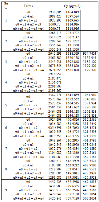
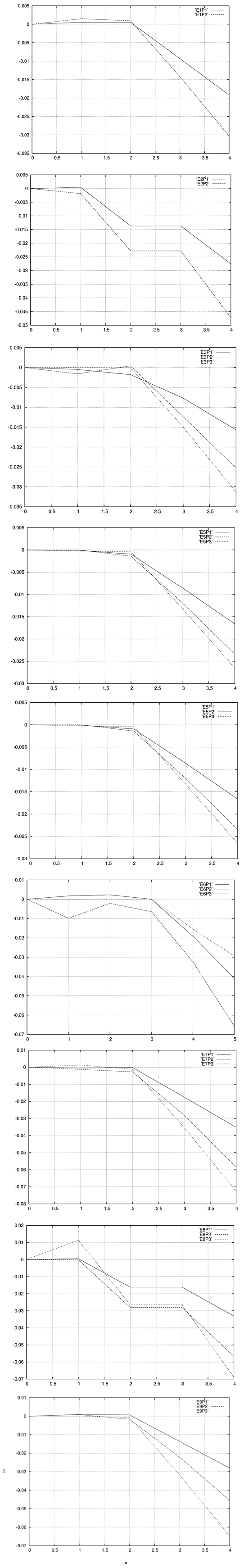Figure 1. Lyapunov exponent λ of Adomian approach depending on the number n of terms for the 9 experiment runs

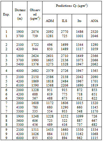
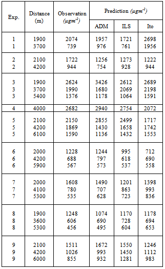
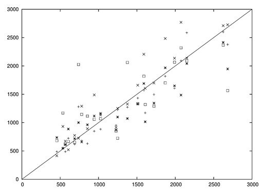Figure 2. Dispersion diagram of predicted (Cp) measured against measured (Co) values by by ADM (+), ILS (×) , Ito (*) e ANA (□)

In figure 3 we show the linear regression of each model, where the closer their intersect is to the origin and the closer the slope is to unity the better is the approach. By comparison one observes that the present approach yields the best description of the data. Details of the regression may be found in table 4.

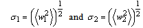
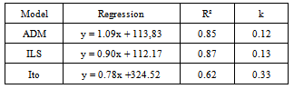
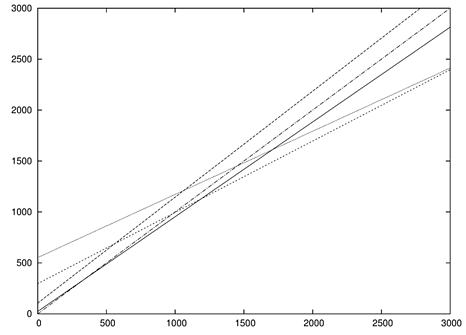Figure 3. Linear regression for the ADM (------), ILS (− − −). Ito (- - -) and ANA (….) with Gaussian pdf. The bisector ( -. -.-.) was added as an eye guide

In order to perform a model validation we introduce an index κ which if identical zero there is a perfect match between the model and the experimental findings.

(13)

Here a is the slope, b the intersection, C_oi the experimental data and the arithmetic mean. Since both the experiment and the model are of stochastic character, fluctuations are present, but in the average model and experiment shall coincide, thus the introduced index represents a genuine model validation.

3.3. Solution for bi-Gaussian Turbulence

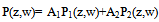
In the convective boundary layer, the heating of the air layer close to the ground produces turbulent flux which gives origin to the so-called up- and down-drafts.

This phenomenon is not symmetric but has a more intensive contribution from the up-drafts. Because of mass conservation the down-drafts occupy a larger area. As a consequence the stochastic term shall be asymmetric which excludes the Gaussian probability density as a convenient function. There is no indication for a unique probability density function so far, nevertheless the following characteristics shall be present.

• The probability density shall have an enhanced tail towards higher velocities, that indicate the more energetic up-drafts, but with a smaller integral proportion than down-drafts.

• The probability density shall have a pronounced maximum at negative velocities, i.e. the down-drafts.

One finds typically two types of asymmetric probability density functions in the literature, the bi-Gaussian and the Gram-Chalier distribution, where the latter is represented by a truncated series of Hermite polynomials.

In the further we discuss the bi-Gaussian probability density function, which contains a linear superposition of two Gaussian functions, one with maximum probability at a positive velocity, the other one at a negative value as for instance in ref.[7].The authors used a pair of Langevin equations, one for up- and one for down-drafts, each with its specific Gaussian function. In this work we condense this phenomenon in one equation, introducing a sum of two Gaussian functions with different parameters and relative weight.

(14)

where A₁ and A₂ define the relative proportions between up- (P₁) and down drafts (P₂) for the vertical turbulent velocities (w).

(15)

Here, m₁, m₂ are the average probabilities of P₁ and P₂, respectively, and σ₁ and σ₂ represent the standard deviations of each distribution. The mean up and down-draft velocities are

(16)

and the respective standard deviations are

(17)

A general prescription on how to determine the parameters A₁, A₂, m₁, m₂, σ₁ and σ₂ consists in the usage of generating functionals of moments.

(18)

From the normalisation and the first four statistical moments one obtains an equation system which eliminates the unknowns.

(19)

(20)

(21)

(22)

(23)

Upon application of the bi-Gaussian probability density function the expression for the deterministic coefficient of the vertical dimension in the Langevin equation is then,

(24)

Using the deterministic coefficient the Langevin equation reads

(25)

where is obtained upon application of the bi-Gaussian probability density function[36]:

(26)

In a more compact form this yields for the Langevin equation with a bi-Gaussian probability density function (25)

(27)

where

(28)

Table 4. Comparison of the linear regressions of ADM, ILS, Ito and ANA for a Gaussian pdf

In Table (5) the concentrations of the measurements together with theoretical predictions of ADM, ILS and Ito are presented. Table (6) shows the numerical convergence of the ADM method. As already evident in the previous case also for the bi-Gaussian probability density function only a few terms are necessary in order to represent a solution.

Figure (5) shows the dispersion plot of the experimental values against the theoretical predicted values by ADM, ILS and the Ito calculus.

We also apply the model validation as introduced in the previous section to the model application with the bi-Gaussian probability density function. One observes that the all three approaches are more or less close to the bisector, however the comparison with the model validation from the previous case shows that the Gaussian probability density function seems more adequate for the stability condition of the experiment which is also manifest in the smallest k for ADM.

From the comparison of the regressions in table 7 one recognizes that the three approaches behave similar with respect to R² but show larger values for k in comparison to the case where the Gaussian probability density function defined the stochastic character of the turbulence.

Table 5. Concentrations from Copenhagen experiment and prediction from ADM, ILS, Ito using a bi-Gaussian pdf

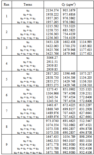
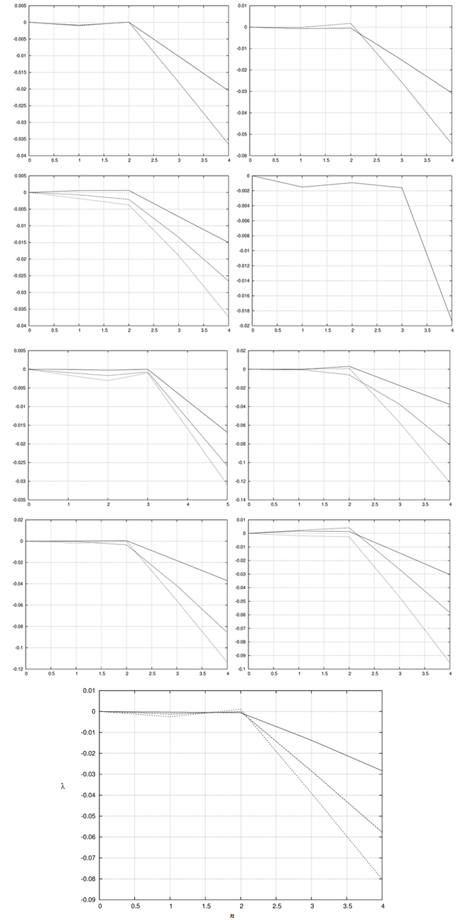Figure 4. Lyapunov exponent λ of the Adomian approach depending on the number n of terms for the 9 experimental runs using the bi-Gaussian pdf.

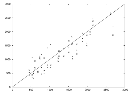Figure 5. Dispersion diagram of predicted (Cp) measured against measured (Co) values by by ADM (+), ILS (×) and Ito (*) for a bi-Gaussian pdf

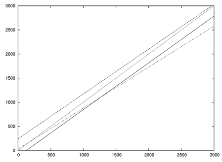Figure 6. Linear regression for the ADM (——), ILS (– – –) and Ito (- - - -) with a Bi-Gaussian pdf. The bisector (– · – ·) was added as an eye guide

Table 6. Numerical convergence of ADM for a bi-Guassian pdf . The multiple columns for Cy refer to the measurements at different distances per run and are given in table 5

Table 7. Comparison of the linear regressions using the bi-Gaussian probability density function Model Regression R2 K ADM y = 0.97x -123.47 0.89 0.10 ILS y = 0.93x +242.34 0.89 0.19 Ito y = 0.85x +29.07 0.86 0.15

3.4. Solution for Gram-Chalier Turbulence

The use of the Gram-Chalier probability density function for stochastic Lagrangian models was proposed by Ferrero and Anfossi (1998)[23] (see also the work by Jensen et al. (1997)[33]), which makes use of an expansion in Hermite polynomials. In the present discussion we use the series until the fourth term resulting in an asymmetric probability density function for the vertical turbulent velocities.

(29)

Table 8. Concentration of the Copenhagen experiment in comparison to the predictions by ADM, ILS and Ito using a Gram-Chalier pdf

where

(30)

(31)

and . In the case of Gaussian turbulence equation (29) recovers the normal distribution with c₃ and c₄ equal zero. The Gram-Charlier probability density function of the third order is obtained by the choice c₄ = 0. Upon application of equation (29) in the equation of the deterministic coefficients yields,

(32)

where j = 1, 2, 3 and is the Lagrangian correlation time scale and and are expressions as shown below.

(33)

(34)

(35)

Inserting the deterministic coefficient (32) into the Langevin equation renders the latter

(36)

Table 9. Numerical convergence of ADM using a Gram-Chalier pdf. The multiple columns for Cy refer to the measurements at different distances per run and are given in table 8

In short hand notation this reads

(37)

where

(38)

(39)

In table (8) we present the concentrations of the Copenhagen experiment together with the results from the ADM, ILS and Ito approaches.

Table 9 shows the numerical convergence of the ADM method. As in the two previous cases only a few terms reproduce with considerable fidelity the exact solution with a Gram-Chalier probability density function.

Figure (8) shows the dispersion plot of observed against predicted data. In Figure (9) are shown the linear regression for the three approaches. All three methods, ADM, ILS and Ito reproduce reasonably well the expected bisector. Using the model validation index k shows that for all three probability density functions the ADM approach yields results closest to the expected concentration profile.

As already mentioned before, the model validation indicates the Gaussian probability density function implemented together with the ADM approach as the most adequate description for the Copenhagen experiment by virtue of k = 0.07 being significantly smaller than all other realizations. This was also to be expected from the stability conditions given in table 10, which characterize the turbulence regime as strong convective.

Table 10. Comparison of the linear regressions for the ADM, ILS and Ito approach using the Gram-Chalier probability density function

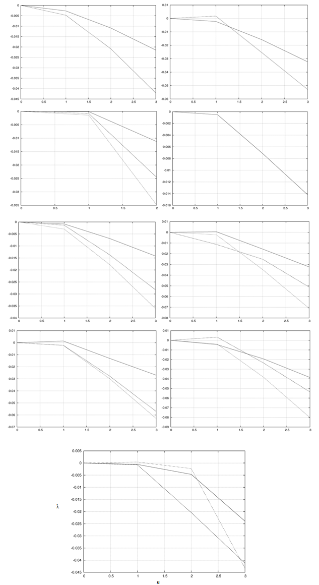Figure 7. Lyapunov exponent λ of the Adomian approach depending on the number of terms n for the 9 experimental runs using the Gram-Chalier pdf

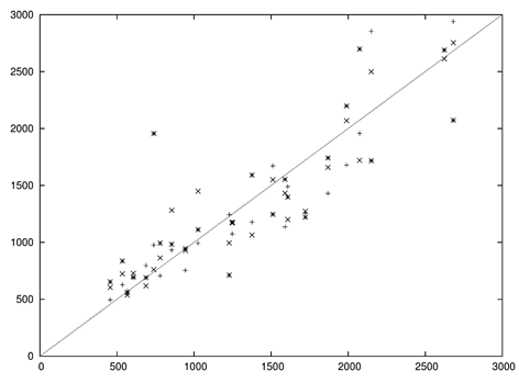Figure 8. Dispersion diagram of predicted (Cp) against observed values (Co) with a Gram-Chalier probability density function

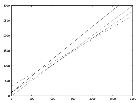Figure 9. Linear regression using the Gram-Chalier probability density function

It is worth mentioning that since convergence is genuinely controlled the present procedure permits to pin down model limitations which in other approaches are hidden in numerical imprecision or approximations.

4. Conclusions

In the present contribution we discussed an approach that is designed to simulate meteorological aspects, that are relevant in eolic park site evaluation. We showed how a realiable model for a turbulent wind profile may be determined among model candidates, that provides the full three dimensional space and time dependent turbulent wind field for an area in consideration.

We showed in a general form how to construct a recursive scheme where convergence is understood. A genuine criterion was introduced based on Lyapunov’s theory, that in our case tests stability of convergence. Application of that criterion showed that in all three cases only five terms are necessary so that the approximate solution differs from the real solution by less than one percent.

On the one hand, the generality of the proposed solution with respect to the considered probability density functions on the other hand the controlled convergence permits to validate the model in question. The resulting model is thus likely to simulate turbulent wind profiles close to those that could be observed in a site in question.

The Gaussian density function yields within the phenomenon inherent fluctuations the best agreement between model and observation. Among the three probability distributions the Gaussian one is from the physics point of view considered the most adequate for the Copenhagen experiment. Thus the criterion to select a model among possible candidates identified the most adequate one.

We believe that we have done a step into a new direction with the present contribution, that may be useful to analyse meteorological aspects as well as simulate possible scenarios, for the purpose of site evaluation, using tracer experiments. Since measurements are typically performed in a limited set of positions a calibrated model is able to reconstruct the three dimensional wind velocity field considering especially the contributions by turbulence. To the best of our knowledge up-to-date the tracer technique is not used for site evaluation, but could supply valuable information on the wind properties for a given region of interest and its time-behaviour.

In this paper we presented an analytical solution of the three-dimensional stochastic Langevin equatioqn applied to tracer dispersion for Gaussian, bi-Gaussian and Gram-Chalier turbulence, respectively. The solution was obtained using the Adomian Decomposition Method (ADM) whose principal advantage relies in the fact that the non-linearity can be taken care of without linearisation or simplifications. Further, the stochastic part is absorbed in the initial term of the iteration and thus propagates through all the subsequent iteration terms. For the Langevin equation the non-trivial questions of uniqueness and convergence for the Adomian approach in stochastic problems is given since the drift and dispersion terms satisfy a Lipschitz condition.