-
Paper Information
- Next Paper
- Paper Submission
-
Journal Information
- About This Journal
- Editorial Board
- Current Issue
- Archive
- Author Guidelines
- Contact Us
American Journal of Environmental Engineering
p-ISSN: 2166-4633 e-ISSN: 2166-465X
2013; 3(2): 100-106
doi:10.5923/j.ajee.20130302.03
Improving the Accuracy of Artificial Intelligence - Based Groundwater Quality Models Using Clustering Technique - A Case Study
 Abstract
 Reference
 Full-Text PDF
 Full-text HTML
Jawad S. Alagha1, Md Azlin Md Said1, Yunes Mogheir2
1School of Civil Engineering, Universiti Sains Malaysia (USM), Nibong Tebal, Pulau Pinang, Malaysia
2Environmental Engineering Department, Engineering Faculty, Islamic University of Gaza, Palestine
Correspondence to: Md Azlin Md Said, School of Civil Engineering, Universiti Sains Malaysia (USM), Nibong Tebal, Pulau Pinang, Malaysia.
| Email: |  |
Copyright © 2012 Scientific & Academic Publishing. All Rights Reserved.
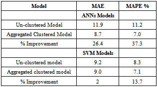
In this study, the simulation performances of two artificial intelligence (AI) techniques – namely, artificial neural networks (ANNs) and support vector machine (SVM) – for groundwater quality modeling were improved by grouping input data into consistent clusters as a pre-modeling technique. AI techniques were applied to model the concentrations of chloride and nitrate using data from the Gaza coastal aquifer in Palestine, which is a very complex hydro-geological system. Research results indicated that developing separate AI models for each cluster reduced the mean absolute percentage errors (MAPE) of the ANNs' models by 20% and 37% for chloride and nitrate, respectively. Meanwhile, the MAPE of the SVM’s models was reduced by 10% and by 13% for chloride and nitrate, respectively. Improving the simulation accuracy of AI techniques would lead to more rational and effective decisions for groundwater management.
Keywords: Artificial Neural Networks (ANNs), Chloride, Clustering, Gaza Coastal Aquifer (GCA), Nitrate, Support Vector Machine (SVM)
Cite this paper: Jawad S. Alagha, Md Azlin Md Said, Yunes Mogheir, Improving the Accuracy of Artificial Intelligence - Based Groundwater Quality Models Using Clustering Technique - A Case Study, American Journal of Environmental Engineering, Vol. 3 No. 2, 2013, pp. 100-106. doi: 10.5923/j.ajee.20130302.03.
Article Outline
1. Introduction
- In the last decade, artificial intelligence (AI) techniques have become highly popular and widely used in modeling hydrological complicated processes using relatively less cost and effort[1]. The superiority of AI techniques becomes apparent when accurately describing the hydrological process is difficult, and when the available data are insufficient to apply numerical and physical models, which is the case for many groundwater (GW) quality problems[2].Recognizing their superior capabilities, the uses of various AI techniques, such as artificial neural networks (ANNs) and support vector machine (SVM), in hydrological applications have considerably increased over the previous decade. For example, ANNs have been successfully applied to different GW applications[3-7]. Likewise, the application of SVM has attracted more attention in recent years for modeling both surface water and GW processes[8-10].Despite the wide strides towards the utilization of AI techniques for GW quality modeling, some areas still require further investigation in this context. Literature revealed that the SVM application for GW modeling is scarcer compared with the growing applications in surface water problems[9]. For example, no study was found to use SVM for modeling the concentration of chloride in GW. Furthermore, with regard to nitrate modeling, none of the earlier studies utilized SVM to estimate nitrate concentration in GW based on the potential influencing variables. As for ANNs, very few applications were found related to model chloride and nitrate concentrations in GW using explanatory variables. In such studies, such as that of Seyam and Moghier[6], the accuracy needs further improvement. On the other hand, studies that were relatively accurate required substantial data input, and utilized sophisticated methods for input calculations; therefore, their applicability could be very limited due to the detailed and accurate data required. An example of such study is that of Almasri and Kaluarachchi[7].In the field of AI applications for GW quality, the simplification of AI models and their improved accuracy without the need for extra data and effort have become the trend. Thus, research on hybrid models that integrate AI with other techniques is considered to be a promising field, with models being developed that use minimum data, time, and effort[11]. These targeted models could then be effectively utilized to support management decisions related to GW quality.This paper aims to improve the simulation performance of ANNs- and SVM-based GW quality models by performing data clustering as a pre-modeling technique. The hybrid systems, composed of AI and clustering techniques, have been applied for modeling both chloride and nitrate concentrations in GW using data from the Gaza coastal aquifer (GCA) in Palestine, which is a very complex aquifer. The improvement of AI simulation performance could in turn lead to more accurate prediction and rational management processes of water resources.
2. Materials and Methods
2.1. Study Area
- The Gaza Strip (GS) area is located at the eastern coast of the Mediterranean Sea (Figure 1 (b)). It is one of the most densely populated areas in the world with an average density of more than 4300 inhabitants/km2; and it is expected that the population density will exceed 5835 inhabitants/km2 in 2020[12]. GS is administratively divided into five governorates, among which Khanyounis governorate which is the study area as shown in Figure 1(c), has the largest area of about 112 km2 with a total population of about 300,000 inhabitants[13]. GS is an extreme model on how unstable political environment, disastrous economic situation, decaying environmental conditions and unplanned human activities are combined together to further deteriorate the GW quality[14].Gaza coastal aquifer (GCA) as shown in Figure 1(a) is the only natural source of water for different purposes in GS. According to UNCT[12] the GW situation in GCA is deteriorating and it could become unusable as early as 2016. GCA suffers from two water quality problems which are the high concentrations of chloride and nitrate[15]. Where, less than 5% of GS municipal water wells meet world health organization (WHO) chloride standards. Moreover chloride concentration in many wells of Khanyounis governorate reached 10 times more than WHO standards[16]. The main sources of the elevated chloride concentration in Khanyounis governorate are seawater intrusion, extensive exploitation, saline water flux from the neighboring eastern Eocene aquifer, and salty water lenses exist in many locations at deeper layers[17]. Likewise, the average nitrate concentration in Khanyounis governorate wells is 191 mg/l which is almost 4 times WHO standards for nitrate[18]. The main sources of the high nitrate levels are disposing of untreated wastewater into the aquifer through cesspits and septic tanks[15]. Additionally agricultural activities where thousands of tons of animal manure and synthetic fertilizers that exceed crop demands are usually applied resulting in leaching the excess nitrogen load into the aquifer[19].
2.2. Data Collection
- Two separate groups of models were developed using potential influencing variables: the first one was related to chloride, while the second, to nitrate. The primary step for modeling water quality using AI techniques is to develop an input-output response matrix between the inputs (potential influencing variables) and outputs (concentration of chemical parameters). Based on the availability of monitoring data, 22 wells that constitute 80% of the municipal wells in Khanyounis governorate were used to develop the AI models. Periodic water quality analyses for municipal wells are usually performed twice a year, in spring (May) and in autumn (November). Chloride and nitrate monitoring data in the case study wells and all associated variables from 2000 to 2010 were collected from the database of the related institutions.
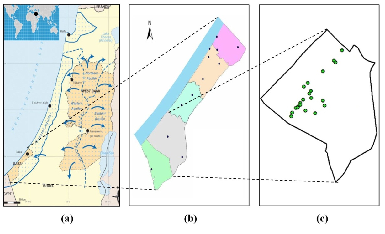 | Figure 1. (a) Gaza Strip and Gaza coastal aquifer layout; (b); Gaza Strip Map; and (c) Location of municipal wells in Khanyounis governorate |
 | (1) |
 | (2) |
3. Results and Discussion
3.1. Clustering of Monitoring Wells
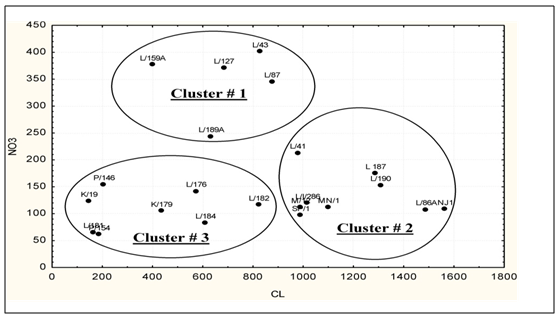 | Figure 2. The concentrations of both Cl and NO3 in case study wells in 2007 for each well’s clusters |
3.2. Modeling of Chloride Concentration
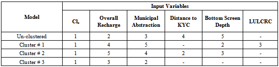
- For ANNs’ models, the architecture that delivered the best results for both un-clustered and aggregated clustered models is the multi-layer perceptron feed forward neural network with one hidden layer. The Levenberg-Marquardt technique provided the best results as a training algorithm. On the other hand, different SVM models were evaluated and optimized until the best performance was achieved. Radial basis function was used as a Kernel function. Table 1 presents the results of the best ANNs and SVM models for chloride. Based on the results, the model’s performance evaluation criteria for the aggregated clustered model were better compared to the un-clustered model, thus indicating the positive effect of well clustering on AI performance. However, the improvement that resulted from clustering in the SVM model was less than that of ANNs.The clustering-induced improvement could be attributed to the fact that the clustering divides the wells into groups that possess a high degree of common characteristics. Accordingly, when separately applying AI technique for each cluster, the model can easily grasp the common variables that affect the output. Moreover, the influence (weight) of each variable on the model’s output is almost the same for all wells at the same cluster. The effect of clustering could be more obvious by investigating the input variables and their order in each separate model, as shown in Table 2. The five input variables of the un-clustered model ordered according to their weights are: Clo, overall recharge, municipal abstraction, distance to Khanyounis center, and bottom screen depth. Meanwhile, for the cluster #1 model, LULC recharge coefficient replaced the distance to Khanyounis center, because almost all cluster #1 wells have the same distance to Khanyounis center; thus, this variable is insignificant for this cluster. Furthermore, built-up areas are the dominant land use for this cluster, and thus the recharge capacity basically depends on the LCLU recharge coefficient. Additionally, the bottom screen depth of the wells in cluster #1 was noted to have the second most significant influence. This observation may be related to the deeper saline water lenses that exist in the locations of cluster #1 wells. Likewise, the input variables of cluster #2 wells are the same as those of the un-clustered model, but possessed different relative weights. These wells have relatively high chloride concentration as compared with the overall mean, and are spatially scattered over the study area. The ranking of the input variables for this cluster shows the three main sources of elevated chloride concentration, which are seawater intrusion, lateral flow, and the effect of saline lenses. The first two sources are expressed by the distance to Khanyounis center, whereas the bottom screen depth indicated the effect of saline lenses. Finally, the input variables of cluster #3 model comprised only Clo, municipal abstraction, and overall recharge, which are the three common input variables for all models. The chloride concentrations in these wells are relatively low, and the wells’ areas are characterized by high GW recharge. Other variables are insignificant because these wells have relatively the same distance to Khanyounis center, and almost all have relatively small bottom screen depths. The results of the best ANNs’ chloride models in this study are indicated higher accuracy than the results obtained by Seyam and Mogheir[6], who developed an ANNs-based model for simulating Cl in GCA. Their result for MAPE was 14%.
|

|
3.3. Modeling of Nitrate Concentration
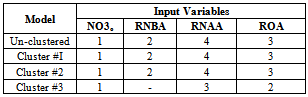
- The architecture that delivered the best results for both un-clustered and aggregated clustered ANNs models was the multi-layer perceptron feed forward neural network with one hidden layer. In addition, the back-propagation and Levenberg-Marquardt training algorithms resulted in the best performance for the various models. For SVM, the different models were evaluated and optimized until the best performance was achieved. Sigmoid and radial basis function were used as a Kernel function. Table 3 presents the results of the best ANN and SVM models for nitrate. The aggregated clustered model has a lower error compared with the un-clustered model for both ANNs and SVM. The improvement of the nitrate model due clustering technique before AI modeling is due to the same reason as that for chloride; that is, the uniform characteristics of the wells falling under the same group, which consequently facilitates the ability of the model to identify the common influencing variables. Table 4 presents the ranking of the input variables for both un-clustered and clustered nitrate models. NO3o produced the largest effect on the nitrate concentration for both clustered and un-clustered models. For the un-clustered models, clusters #1 and #2, the second, third, and fourth influencing input variables were recharge and N-load from built up areas, recharge from open areas, and recharge and N-load from agricultural areas respectively. However for cluster #3, recharge and N-load from built up areas was not included in the model. Ranking the input variables for each developed model demonstrated the effect of LULC on GW nitrate concentration. For instance, recharge and N-load from built up areas was insignificant in cluster #3 wells because the average built up area around the wells of this cluster was less than 5%. Therefore, the effect of the built up areas was limited. On the other hand, the area of the three LULC categories for un-clustered, cluster #1, and cluster #2 models were considerable. Therefore, all categories are significant input variables in the models. The results of nitrate modeling are comparable with those of other similar studies. For example, Almasri and Kaluarachchi[7] modeled nitrate concentration in the Sumas-Blaine aquifer of Washington, United States using ANNs and achieved a 6.7% MAPE. They utilized highly accurate maps with 21 LULC categories. Moreover, they used a relatively sophisticated method in identifying the well’s buffer zone. By contrast, the present study used low quality aerial photos in classifying the entire study area into three LULC categories, using an easy method for the well’s buffer zone delineation. The results of this research are relatively more accurate than those obtained by Almahallawi et al.[24], wherein the model’s MAPE was 8.43%. With regard to the comparison between ANNs and SVM, the research results are largely consistent with those obtained by Dixon[10], who used both techniques to differentiate between the wells that were contaminated and uncontaminated by nitrate. He reported that ANNs outperformed the SVM, especially on training data. Nevertheless, the results of both techniques were comparable for the test data set.The accuracy of the nitrate models (MAPE = 7.0%) was less than that of chloride model (MAPE = 3.7%). This result may be attributed to the high complexity of the GW contamination by nitrate. The nitrate simulation results are mainly affected by LULC categories, which were obtained through an analysis of aerial photos, and the quality of the aerial photos played a crucial role. Moreover, the calculations of input variables were based on an estimation of the average N-load and recharge for each LULC, which are not always accurate. Other variables, such as bacterial role in nitrification and de-nitrification processes, may likewise affect simulation accuracy. On the other hand, the values for most of the input variables for the chloride model were specific and accurate, including the abstraction quantities, distance to Khanyounis center, as well as the depth of the well’s bottom screen.
|
|
4. Conclusions
- Assessment of the effect of the wells’ clustering technique in improving the simulation performance of AI-based GW quality models in complex aquifers as conducted in this study indicated that the clustered models outperformed the un-clustered models. This result indicates the effectiveness of wells’ clustering as a pre-modeling technique on AI models’ performance, especially for ANNs. AI models for each distinct cluster captured the input-output relationships more accurately due to the similarity of the characteristics of wells grouped under the same cluster. The improvement of the AI models due to data clustering is obvious, even though the clustered models have less data sets compared with the un-clustered model, which adversely affected the model’s performance. Consequently, clustering the sampling points and stations before applying AI techniques particularly for heterogeneous systems is highly recommended. However, the number of clusters must be kept to a minimum, such that data scarcity associated with clustering does not affect the model’s performance.Introducing a comprehensive and periodic GW monitoring system is never an easy task, owing to various financial and technical constraints in many regions of the world, particularly in developing countries. Thus, accurately modeling the most sensitive and dominant GW quality parameters using cost-effective techniques that rely on few monitoring data presents a highly advantageous opportunity, as setting rational GW management strategies depend on the availability of accurate, applicable, and reliable simulation models. Therefore, the importance of the present study stems from the growing need to improve the accuracy of the GW quality model, without requiring additional data and effort. The clustering technique does not require extra data, apart from routine monitoring data. Consequently, the accurate, simple, and applicable AI models developed in this study can be applied in setting appropriate strategies and making rational decisions related to GW management.