Lenise Saraiva 1, Nisia Krusche 2
1Programa de Pós Graduação em Modelagem Computacional, Universidade Federal do Rio Grande, Rio Grande, 96203-900, Brasil
2Centro de Ciências Computacionais, Universidade Federal do Rio Grande, Rio Grande, 96203-900, Brasil
Correspondence to: Nisia Krusche , Centro de Ciências Computacionais, Universidade Federal do Rio Grande, Rio Grande, 96203-900, Brasil.
| Email: |  |
Copyright © 2012 Scientific & Academic Publishing. All Rights Reserved.
Abstract
Understanding the behavior of the planetary boundary layer is fundamental to better comprehend some phenomena such as the dispersion of pollutants in urban areas. This study aims at estimating the characteristic parameters and the spectral properties of the atmospheric turbulence on the surface boundary layer, especially the height of the atmospheric boundary layer in the south of Rio Grande do Sul state, in Brazil, based on data collected by micrometeorological instruments placed close to the surface. The characteristic parameters and the spectral properties were analyzed in the light of Monin-Obukhov’s similarity theory in different stability conditions. The boundary layer height was determined by using the turbulent spectra of the zonal wind velocity whose data was collected from August 28th to November 11th, 2006, on a tower located 20 km south of Rio Grande. Results of the turbulence kinetic energy, the friction velocity and Obukhov’s length are in agreement with the findings of other studies carried out in the region. After making adjustments regarding the atmospheric stability, the roughness length properly represented the characteristics of the landscape in the region where the data collection tower was placed. The spectral analysis showed that Monin and Obukhov’s similarity theory is not appropriate to describe the spectral characteristics of the turbulence in the somewhat unstable conditions in the region. Mean values of 1168.87 m and 291.90 m were obtained for the heights of the convective and the nocturnal boundary layers, respectively. The methodology that was used to estimate the boundary layer height was satisfactory to represent both its diurnal and its nocturnal evolution.
Keywords:
Atmospheric Turbulence, Turbulent Spectra, Boundary Layer Height
Cite this paper: Lenise Saraiva , Nisia Krusche , Estimation of the Boundary Layer Height in the Southern Region of Brazil, American Journal of Environmental Engineering, Vol. 3 No. 1, 2013, pp. 63-70. doi: 10.5923/j.ajee.20130301.09.
1. Introduction
Variations of the boundary layer characteristics over time, due to seasonal changes and other local influences, are important especially to understand the impact of the dispersion of pollutants in a growing industrial region, which has an important harbor in the southern region of Brazil. It is located at the coastal plains of Atlantic Ocean, which is a geographic boundary to the southwest. The coastal plains in the southern region of Brazil are dotted by lakes and lagoons of various sizes. The largest one is the Patos Lagoon, which stretches over 400 km, and is located to the north of Rio Grande. To the southeast, there is the Mirim Lagoon, on the border with Uruguay, which is connected to the Patos Lagoon by the São Gonçalo channel.Those water bodies generate several local circulations, such as lake and ocean breezes, which interact to the larger scale circulations. They also have an impact in the evolution of the boundary layer.The boundary layer height is a length scale that characterizes the structure and evolution of the planetary boundary layer. Therefore it is of great importance in the determination of functions that express in a universal way the physical processes that happen in it.The results of the classical experiments in Kansas (1968) and in Minnesota (1979) were essential to establish a framework to the description on turbulence on the Planetary Boundary Layer, based on Fourier’s spectra analysis. Some adimensional parameters for homogeneous surfaces and for different stability conditions were derived from these analysis and are generally accepted as standard[1]. Nevertheless, few experiments have been carried out in Brazil to determine the characteristics of atmospheric turbulence, according to[2].Therefore, we aimed at studying the atmospheric turbulence in the Boundary Layer in a region in the south of Rio Grande do Sul state, which is the southernmost state in Brazil. We analyzed high frequency surface data to estimate the height of the boundary layer in this region under different atmospheric conditions.
2. Data
The period of measurement was from August 28th to November 11th, 2006. The site location was about 20 km south of Rio Grande, at 32o 05’ S and 52o 25’ W. The São Gonçalo channel crosses some hundred meters to the northwest of the site, to the southeast there is the Mirim Lagoon, and to the North and northeast, the Patos Lagoon, as shown in Figure 1.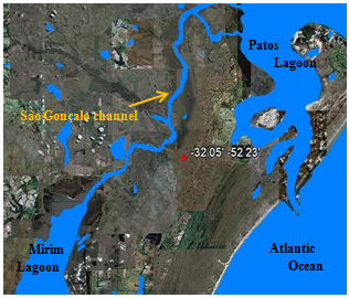 | Figure 1. Region surrounding Rio Grande town, the location of the site is the red dot |
The region is a homogenous and very flat land, with no obstacles for about 500 m in all directions around the tower location, except for a large 3 m irrigation channel which runs from West to East, to the North. There are also some small irrigation channels to the southeast, as shown in Figure 2.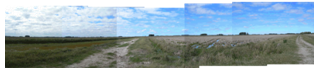 | Figure 2. The land around the site, from the northeast to the south; sand roads take to the east and to the south |
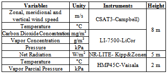
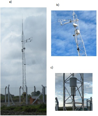
The instruments and the height at which they were attached to the tower are in Table 1. There was a triaxial anemometer, a carbon dioxide and vapor analyzer, a net radiometer, and a sensor of temperature and humidity. The height of the tower was 10 m (Figure 3). The data was stored in a CR5000 Campbell datalogger, and the measurements were made at a frequency of 20 Hz.Table 1. Variables, their unities, the instruments used to measure them, and the height at which they were attached
 |
| |
|
 | Figure 3. a) Tower, surrounded by fence, the dog house was protecting the spare battery, b) triaxial anemometer and carbon dioxide and vapor analyzer on the top, while net radiometer is below, and c) sensor of temperature and humidity |
3. Methodology
Firstly, some characteristic parameters (such as the turbulence kinetic energy, the friction velocity and the roughness length) and the spectral properties of the atmospheric turbulence on the surface boundary layer were determined in different stability conditions in the light of the Monin-Obukhov’s similarity theory which considers a horizontally homogeneous and almost stationary flow and constant turbulent heat fluxes and momentum.A measurement of the intensity of the turbulence may be given by the turbulence kinetic energy. According to the statistical theory of turbulence, irregular behavior of physical values may be expressed as a mean value and a statistical fluctuation around that value (Stull, 1988). Therefore, the zonal (u), meridional (v) and vertical (w) components of the wind velocity may be described as: | (1) |
where  and
and  are the mean components and
  and
and  are the turbulent components.As a result, Turbulence Kinetic Energy (TKE) may be defined as:
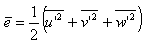 | (2) |
Friction velocity was obtained by Reynolds stress tensor, which considers the vertical transport of both the longitudinal momentum and the transversal momentum. 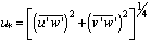 | (3) |
Where  and
and  are the wind turbulent vertical fluxes of components u and v, respectively.The roughness length, z0, characterizes the roughness of the land; it is defined as the height above the ground where velocity is zero, in theory[3]. Roughness length was estimated by using the adjusted logarithmic wind profile. The effects of the variation of the atmospheric stability are introduced in the equation by ψM[1]. The wind velocity is thought to vary with the height in agreement with the logarithmic profile in the following equation:
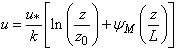 | (4) |
where u* is the friction velocity, zo is the roughness length, k is von Karmam constant (k=0.4), u is the intensity of the average wind and z is the measurement level. The function  is given, in stable conditions, by
 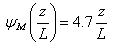 | (5) |
and, in unstable conditions, by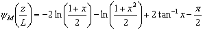 | (6) |
where  Fourier transform was then applied to data on wind velocity, following the steps suggested by[3], to obtain the turbulent spectra.Afterwards, the spectra were normalized by the friction velocity and by the dissipation rate; adjustment curves for the turbulent spectra were also defined. In micrometeorology, analytical expressions are used to represent the spectra, such as:
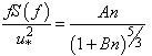 | (7) |
 | (8) |
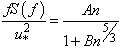
where A and B are constants that only affect the position of the spectrum, rather than its shape[4]. The most common spectral shapes are the neutral spectra from the Kansas experiment[4]. Equation (7) shows a better adjustment to the zonal and meridional components of the wind velocity whereas Equation (8) shows a better adjustment to the vertical component, as follows: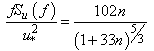 | (9) |
 | (10) |
 | (11) |
The determination of the boundary layer height was carried out by the spectra of the horizontal components of the wind velocity, in agreement with the methodology applied by[5]: wave lengths of the spectral peaks for components u and v are proportional to the boundary layer height. To determine the heights of the nocturnal and convective boundary layers, the wave lengths of the spectral peaks for components u and v[(λm)u and (λm)v] were considered to be proportional to zi (Kaimal et al., 1976), as follows: | (12) |
The resolution of this problem requires the determination of the maximum spectral peak associated with these components. To determine the spectral peaks, dimensionless frequencies, obtained by curves adjusted to the spectra, were used. The maximum wave length (λm) was obtained by  , where nm is the dimensionless frequency of the maximum.According to[6] apud[5], the estimation of the height of the stable ABL is given by:
 | (13) |
This equation can only be applied to very flat land.
4. Results and Discussion
Firstly, the intensity and the direction of the wind velocity were determined by using the mean data on the zonal and meridional components of the wind velocity collected in the experiment. Figure 4 shows the frequency distribution of the wind direction related to the intensity of the wind velocity; it is noteworthy to mention that the NE direction was predominant when the experiment was conducted and that the highest intensities were mostly related to winds that blow in that direction. 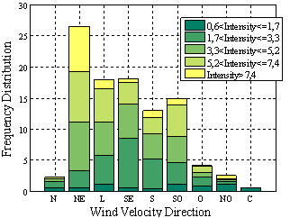 | Figure 4. Frequency distribution of the wind velocity direction, according to its intensity, in m / s |
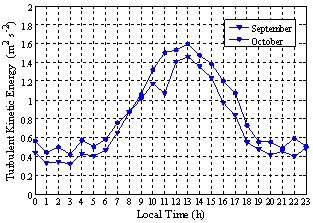
Similar results were found by[7] in his study of the temporary climate normals in Rio Grande from 1991 to 2000. The characteristics of the structure of the surface boundary layer were then analyzed by applying the Monin-Obukhov’s similarity theory in different stability conditions. Parameters, such as the turbulence kinetic energy (TKE), the friction velocity (u) and the roughness length (z0) were determined for every data file. Figures 5 and 6 show the monthly mean behavior of the turbulence kinetic energy and the friction velocity. The highest values of turbulence kinetic energy and friction velocity were observed in October. Studies carried out by[8] recorded, on average, lower values of turbulence kinetic energy and friction velocity in spring, in a more continental area, than the findings we have obtained. Figure 7 shows the roughness length which was determined by using the expression of the logarithmic wind profile and the values of the roughness length which were adjusted to the atmospheric stability. Results were in agreement with values estimated for low vegetation, according to[3], who recorded lengths below 0.2 m in 96.64% . 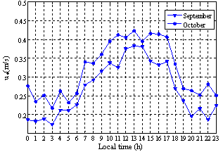 | Figure 5. Hourly average of the turbulent kinetic energy for the months of September and October |
 | Figure 6. Average hourly friction velocity for the months of September and October |
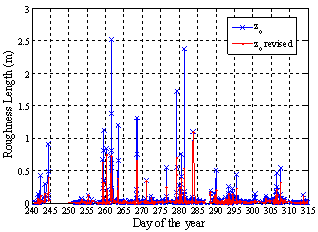 | Figure 7. Temporal variation of roughness length, calculated by the wind logarithmic profile and roughness length, taking into account atmospheric stability |
The analysis of the roughness length in relation to the direction of the wind velocity (Figure 8-a) showed that there were higher values at 3600. It may have happened due to the fact that the topography comprises a large irrigation channel in this sector, as shown in Figure 8-b.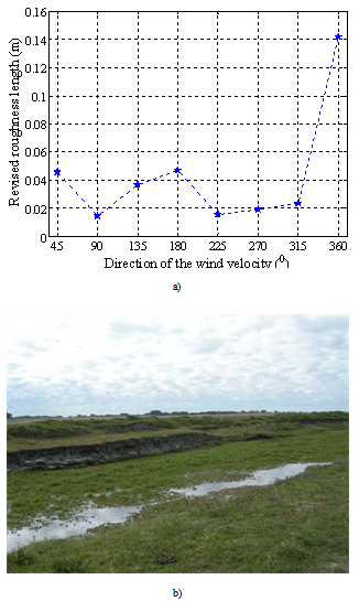 | Figure 8. a) Roughness length adjusted to the direction of the wind velocity (average per sector) and b) View at 3600 |
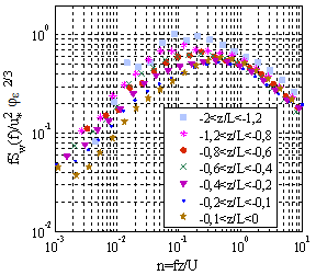
The spectral analysis usually requires mean periods of 60-90 minutes[1]. Tests were carried out in shorter periods (20 minutes), however, the spectra did not show clear positions for the energy peak. Thus, the spectral analysis was conducted in 60-minute periods, on average, for all 930 series of data. Since the frequency of data acquisition was 20 Hz, every 1-hour series has 72000 points. Figure 9 shows the spectrum of the vertical wind velocity (w) in one case with stable conditions and one with unstable conditions, besides the smoothing of 22 frequency bands. The law of –5/3 was observed in the inertial subinterval. The spectra were normalized by the friction velocity and by the dissipation rate. The region of the inertial subinterval can be clearly identified for the mean spectra in the unstable period and the grouping of all spectral curves can be observed for a -2/3 slope (Figure 10). In the stable period (Figure 11), only the curves that represent more stable series show this grouping. 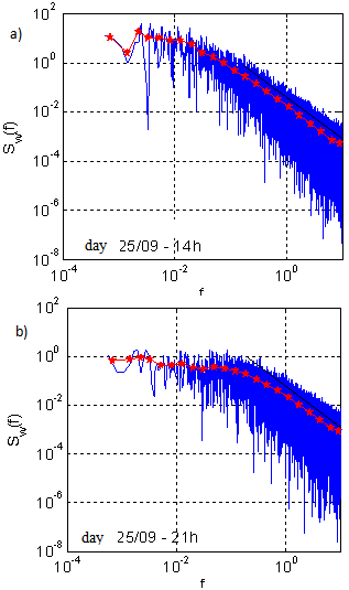 | Figure 9. Turbulent spectrum of the vertical wind velocity in a) unstable period and b) stable period,; the red curve represents the smoothing in 22 bands and the straight line represents the law of –5/3 in the inertial subinterval |
 | Figure 10. Mean spectrum of the wind vertical velocity in the unstable period |
 | Figure 11. Mean spectrum of the wind vertical velocity in the stable period |
We observed an anomalous behavior of the mean spectrum of the wind vertical velocity in regions with high frequencies. The spectra tend to increase in these regions, after the fall. This phenomenon is called aliasing and may happen to any data series in two cases: when the sampling rate is superior to capacity the sensor has to measure in terms of response time and when the frequency of the physical process is higher than the measurement rate[3]. At the end of low frequencies, mainly for the spectra in the stable period, behavioral distortions are also observed. According to[1], these distortions result from trends in the temporal series; they can be defined as any frequency component whose period is higher than the length of the data recording. Adjustment curves were obtained by (7). Constants A and B suggested by[4] for the adjustment curves of the normalized spectrum of the vertical wind velocity were tested and adjusted for the data series under investigation. As an example of the results obtained for the smoothed spectra and their adjustment curves, Figure 12 shows a case in stable conditions and one in unstable conditions. 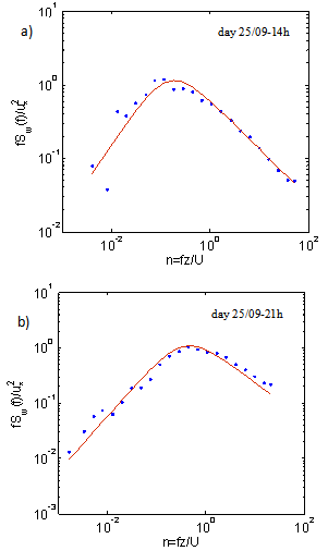 | Figure 12. Example of the smoothed turbulent spectra fit of the vertical wind velocity component normalized by u * for a) unstable conditions and b) stable conditions |
Figure 13 shows the mean adjustment curves in different stability conditions related to the dimensionless frequency. The ordination that follows the variation of the stability parameter and the separation into regions with unstable and stable spectra can be observed.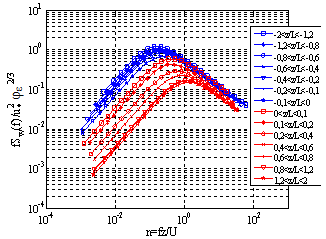 | Figure 13. Mean fit for different stability conditions |
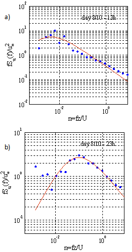 | Figure 14. Example of smoothed turbulent spectra fit of the zonal wind speed normalized by u * for a) unstable conditions and b) stable conditions |
A study of atmospheric turbulence carried out by[8] provided evidence of the efficiency of Monin-Obukhov’s similarity theory when it was applied to data collected during the first meteorological experiment in Rio Grande in March 2002. To estimate the height of the boundary layer, only the spectra of the zonal wind velocity (u) were analyzed because it is the predominant wind in this region.Adjustment curves were obtained by (8). Constants A and B suggested by[4] for the adjustment curves of the normalized spectrum of the zonal wind velocity (9) were tested and adjusted to the data series under investigation, just like for the spectra of the vertical component of the wind.Figure 14 shows a case in stable conditions and one in unstable conditions as an example of results obtained for the smoothed spectra and their adjustment curves. The height of the nocturnal boundary layer (stable period) ranged approximately between 100 m and 300 m. However, the height of the convective one (unstable period) has high variation even though its maximum height does not exceed 1800 m (Figure 15).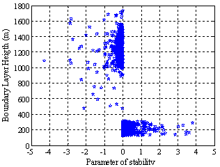 | Figure 15. Variation of the boundary layer height due to atmospheric stability |
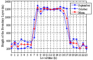 | Figure 16. Average hourly height of the boundary layer for the months of September and October and the average hourly total for those months |
Figure 16 shows the hourly means in September and October and the mean in both months.The height of the mixture layer is deeper in October than in September. In the stable period, however, on average, the height of the layer is deeper in September than in October. Mean values of 1168.87 m and 291.90 m were obtained for the convective and the nocturnal boundary layers, respectively. Some authors[10] estimated some parameters that characterize the atmospheric turbulence in Candiota, RS, by using a numerical model. As a result, the height of the convective layer did not exceed 1000 m and the height of the nocturnal layer was about 200 m. Values close to the boundary layer height in different studies show coherence in both studies since both use indirect measurements.
5. Conclusions
This research analyzed temporal series collected at a 20 Hz frequency in the south of Rio Grande do Sul state to study the behavior of the atmospheric turbulence in the region. The turbulence kinetic energy was calculated and some characteristic parameters, such as the friction velocity and the roughness length, were determined in agreement with the Monin-Obukhov’s Similarity Theory in different stability conditions. Results were satisfactory. The roughness length took into account the stability parameter and properly represented the topography of the region where the data collection tower was placed. For the spectral analysis, spectra were determined by using mean 60-minute periods because they had clearer positions for the energy peak. The law of –5/3 was observed in the inertial subinterval for the spectra of the vertical wind velocity. In unstable conditions, the spectra were satisfactorily normalized by the friction velocity and the dissipation rate. The region of the inertial subinterval and the convergence of all spectral curves to a -2/3 slope were clearly identified. However, in stable conditions, only the curves that represented more stable series were satisfactorily normalized and fell. For the stable series closer to neutrality, the scales of the Monin-Obukhov’s Similarity Theory did not prove to be appropriate or sufficient to describe the spectral characteristics of the turbulence. The methodology that was used to estimate the boundary layer height by the spectra of the horizontal components of the wind velocity was satisfactory to represent both its diurnal and its nocturnal evolution.
ACKNOWLEDGEMENTS
The authors would like to thank Osvaldo L. L. Moraes, Ph. D., for providing the program that generates the smoothed spectral densities and CNPq, for the support and the funds for this research.
References
| [1] | J. C. Kaimal, J. J. Finnigan, “Atmospheric Boundary Layer Flows: Their Structure and Measurement”, Oxford University Press, New York, 289 pp, 1994. |
| [2] | R. Magnago, G. Fisch, O. Moraes, “Análise espectral do vento no Centro de Lançamento de Alcântara (CLA)”, Revista Brasileira de Meteorologia, v.25, n.2, 260 - 269, 2010 |
| [3] | R. B. Stull, “An Introduction to Boundary Layer Meteorology”, Kluwer Academic Pub., Dordrecht, Holanda. 1988. |
| [4] | J. C. Kaimal, J. C. Wyngaard, Y. Izumi, O. R. Coté, “Spectral Characteristics Of Surface-Layer Turbulence”, Quart. Journal R. Meteorological Society, 98, 563-589. 1972. |
| [5] | J. E. Lamesa, “Estudo espectral da camada limite superficial de Iperó, SP”, Master’s Thesis, Instituto de Astronomia, Geofísica e Ciências Atmosféricas da Universidade de São Paulo. São Paulo, 2000. |
| [6] | F. Pasquill, F. B. Smith, “Atmospheric Diffusion”, 3a ed., Ellis Horwood Ltd. Chichester, England, 437 pp. 1983. |
| [7] | M. S. Reboita, “Normais Climatológicas Provisórias de Rio Grande, RS, no Período de 1991 a 2000”, Monograph in Geography. Universidade Federal do Rio Grande. Rio Grande, 2001. |
| [8] | O. L. L. Moraes, “Turbulence Characteristics in the Surface Boundary Layer over the South American Pampa”, Kluwer Academic Publishers, Boundary- Layer Meteorology, 96, 317-335, 2000. |
| [9] | L. B. Saraiva, N. Krusche, “Estudo da Turbulência Atmosférica Durante o I Experimento Meteorológico de Rio Grande”, Revista Ciência e Natura, III Workshop Brasileiro de Micrometeorologia: 207 – 210, 2003. |
| [10] | F. S. Puhales, “Estudo do Ciclo Diário da Camada Limite Planetária Através da Simulação dos Grandes Turbilhões”, Master’s Thesis. Programa de Pós-Graduação em Física da Universidade Federal de Santa Maria. Santa Maria, RS. 2008 |
 Abstract
 Reference
 Full-Text PDF
 Full-text HTML