1. Introduction

A general mathematical theory for dealing with inverse problems is due to the Russian mathematician Andrei Nikolaevich Tikhonov at 1963, introducing the regularization method as a general procedure to solve such mathematical problems. The regularization method looks for the smoothest (regular) inverse solution, where the data model would have the best fitting related to the observation data, subject to constrains. The searching for the smoothest solution is an additional information (or “a priori” information), which reads the ill-posed inverse problem a well-posed one[1]. In the mathematical implementation of the method, the inverse problem is formulated as an optimization problem with constrains (a priori information). These constrains can be added to the objective function with the help of a regularization parameter:

(1)

being u the unknowns, A(.) the mathematical model, the observation with δ noise level, Ω(.) the regularization operator, and α the regularization parameter.

This paper is focused on the application of inverse prolem methodology for solving a problem with strong interest in meteorology and environmental science: estimation of the emission rate from the area pollutant sources. The identification of the pollution source is calculated here obtaining a regularized inverse solution.

The problem for identifying the minority gas emission rate for the system ground-atmosphere is an important issue for the bio-geochemical cycle, and it has being intensively investigated. This inverse problem has been solved using regularized solutions[2], Bayes estimation[3, 4], and variational methods[5] – the latter approach coming from the data assimilation studies.

In principle, we have no information about how the area pollution source emission rate is spatially distributed. Seibert[6] and other researchers have suggested a domain decomposition, where each sub-domain has different pollutant emission strength. The direct problem can be expressed as forward-time evolution problem, or even as in a backward-time pollutant diffusion problem. The choice between these approaches (forward-time or backward-time) is given by the proposed scheme that has lower computational effort. The decision is based on the number of sources and number of the measurement points. If the number of receptors is less than the number of sources, the backward-time approach should be adopted; otherwise (if the number of receptors is greater than number of sources) the forward-time approach is suggested.

In this study, the direct mathematical model is described by a Lagrangian particle stochastic code. However, here the direct model is represented by the source-receptor scheme. In such approach, the measured concentration in a given receptor is calculated from the contribution of all sources by means of a transition matrix. The entries of the transition matrix are determined employing the Lagrangian code. Therefore, the direct model is represented by a matrix-vector product, instead of use the very expensive Monte Carlo Lagragian scheme for each iteration of the optimization process. This procedure reduces the computational effort (complexity) of the inverse analysis.

The inverse problem is formulated as a constrained nonlinear optimization problem and solved by a quasi-Newtonian optimization algorithm. The objective function is the norm L₂ (see equation (1)) of the differences between the measured concentration and the concentration computed from the mathematical model (Lagrangian code), associated to the regularization operator. The regularization operator for the objective function (1) is the entropy measure of the vector of second-differences of the unknown parameters. This constrains the class of solution candidates into a restricted set of values composed by global smooth sub-domains, similar to the second-order polynomial surface. This regularization approach has been successfully adopted to retrieve the vertical atmospheric profile from satellite data[7], and to identify the turbulent eddy diffusivity[8].

The use of maximum entropy principle to reconstructing sources of inert atmospheric tracers from measurements have been independently introduced by[9] – see also[10] and[11] – an application of the Bocquet’s scheme for reconstruction of the Chernobyl accident source term is described by Davoine and Bocquet[12], for both papers the forward model is given by an Eulerian approach.

In a previous study on higher entropy regularization, it was shown that Morosov’s discrepancy principle was really efficient for the problem of determining the regularization parameter[13]. Here, another method to select the regularization parameter is explored.

The next section is a brief presentation of the formulation of the direct problem. This is followed by a description of the proposed inversion method, and a discussion of the numerical examples. The method is tested over a two-dimensional domain, using synthetic data corrupted with Gaussian white noise.

2. LAMBDA: the Lagrangian Stochastic Model

The Lagrangian particle model LAMBDA was developed to study the transport process and pollutant diffusion, starting from the Brownian random walk modeling[14, 15]. In the LAMBDA code, full-uncoupled particle movements are assumed. Therefore, each particle trajectory can be described by the generalized three dimensional form of the Langevin equation for velocity[16]:

(2a)

and

(2b)

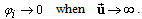
where , and x is the displacement vector, U is the mean wind velocity vector, u is the Lagrangian velocity vector, a_i(x,u,t) is a deterministic term and b_ij(x,u,t)dW_j(t) is a stochastic term, and the quantity dW_j(t) is the incremental Wiener process.

The deterministic (drift) coefficient a_i(x,u,t) is computed using a particular solution of the Fokker- Planck equation associated to the Langevin equation. The diffusion coefficient b_ij(x,u,t) is obtained from the Lagrangian structure function in the inertial subrange, (τ_K << Δt << τ_L), where τ_K is the Kolmogorov time scale and τ_L is the Lagrangian de-correlation time scale. These parameters can be obtained employing the Taylor statistical theory on turbulence[17].

Backward integration can also be applied. This is just to identify which particle arriving in a sensor-j is coming from a source-i.

The drift coefficient a_i(x,u,t), for forward and backward integration is given by

(3a)

with,

(3b)

and

(3c)

where c_v=1 for forward integration and c_v=–1 for backward integration, P_E=P(x,u,t) is the non-conditional PDF of the Eulerian velocity fluctuations, and B_ij = (1/2)b_ikb_jk. Of course, for backward integration, the time considered is t’=–t, and velocity U’=–U being U the mean wind speed. The horizontal PDFs are considered Gaussians, and for the vertical coordinate the truncated Gram-Charlier type-C of third order is employed[15].

The diffusion coefficients, b_ij(x,u,t), for both forward and backward integration are given by

(4)

where δ_ij is the Kronecker delta, σ_i² and τ_Li are velocity variance at each component and the Lagrangian time scale[17], respectively. With the coordinates and the mass of each particle, the concentration is computed – see equations (5) and (6).

The inverse problem here is to identify the source term S(t). As mentioned, a source-receptor approach is employed for reducing the computer time, instead of running the direct model (equation (2)) for each iteration. This approach displays an explicit relation between the pollutant concentration of the i-th receptor related the j-th sourcers:

(5)

where the matrix M_ij is the transition matrix, and each matrix entry given by

(6)

where V_R,i and V_S,j are the volume for the i-th receptor and j-th source, respectively; N_S,j and N_R,i are the number of particle realised by the j-th source and i-th sensor, respectively; N_R,i,j and N_s,i,j are the number of particle released by the j-th source and detected by the i-th receptor.

3. Inverse Model

In order to set up the inverse analysis, it is assumed that the concentration obtained with a mathematic model is given by C^Mod(r,Q), where Q=[Q₁(t), Q₂(t), … , Q_n(t)]^T is the vector emission rate, and Q_n(t) represents the emission rate of the n-th source and C^Exp(r) are data from measurement concentrations. The solution of an inverse problem is a function Q hat minimizes the following objective function:

(7)

with Ω begin a regularization function and α a positive parameter, i.e. a Lagrange multiplier. Each source emission lies in the interval: Q_i ∈[l_i , u_i]. The lower bound l_i and the upper bound u_i are chosen to allow the inversion to lie within some physical limits. The least square difference between experimental data and the computed values is represented by

(8)

The regularization operator can be expressed by an entropic scheme[7, 8, 13]

(9a)

(9b)

with

(9c)

and Q^(m) represents the m-th derivative or difference among the unknown function or parameter vector. The application of derivative or difference operators is associated with whether we are dealing with continuous function or a discrete one. The function S^(m) attain its global maximum when all k(r) are the same, i.e., a uniform distribution, in contrast, the lowest entropy value k_min=0 is reached when the probability distribution from the k(r) is a Dirac delta. This scheme is based on Jaynes’ criterion of inference[18], called maximum entropy principle (MaxEn-0).

Many schemes have been proposed to find the value of the regularization parameter. This parameter provides a fine balance between the square difference and the regularization terms. Some of these techniques are: Morozov’s discrepancy principle[19, 20], the L-curve[21], and the generalized cross validation[20].

3.1. Optimization Algorithm

The optimization problem is iteratively solved by the deterministic method: quasi-Newtonian optimizer routine E04UCF[22], from the NAG Fortran Library. This routine is designed to minimize an arbitrary smooth function subject to constraints (simple bounds, linear and nonlinear constraints), using a sequential programming method. For the n-th iteration, the calculation proceeds as follows:

1. Solve the direct problem for Sⁿ and compute the objective function J(Sⁿ).

2. Compute by finite differences the gradient ∇J(Sⁿ).

3. Compute a positive-definite quasi-Newton approximation to the Hessian Hⁿ:

(10)

where

4. Compute the search direction dⁿ as a solution of the following quadratic programming subproblem:

Minimize , subjected to:

5. Set, Sⁿ⁺¹ = Sⁿ + βⁿdⁿ where the step length βⁿ minimizes J(Sⁿ + βⁿdⁿ).

6. Test the convergence; stop or return to Step 1.

4. Numerical Experiment

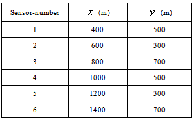
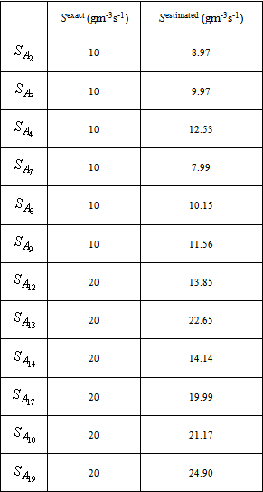
For testing the procedure to estimate the emission rate procedure, the area pollutant sources are considered as placed in a box volume, where the horizontal domain and vertical height are given by: (1500 m 1000 m) 1000 m. There are two embedded regions R₁ and R₂ into a computational domain, with the following horizontal domain (600 m 600 m) for each region, and 1 m of height, and they are realising contaminants with two different emission rates. Figure 1 shows the computational scenario in a two-dimensional projection (x,y): the six sensors are placed at 10 m height and spread horizontally with the coordinates presented in Table 1. The domain is divided into sub-domains with 200 m 200 m 1 m. The emission rates for each sub-domain (S_Ai) are as follows,

R₁ = S_A2 = S_A3 = S_A4 = S_A7 = S_A9 = 10 gm^-3s^-1 ,

R₂ = S_A12 = S_A13 = S_A14 = S_A17 = S_A18 = S_A19 = 20 gm^-3s^-1 .

For other sub-domians: S=0. The dispersion problem is modelled by the LAMBDA backward-time code, where data from the Copenhagen experiment are used, for the period (12:33 h – 12:53 h, 19/October/1978)[23, 24] It is assumed a logarithmic vertical profile for the wind field

(11)

being U(z) the main stream, u_* the fiction velocity, κ the von Kármán constant, z the height above the ground, and z₀=0.06 m the roughness. The wind speed was measured at 10 m, 120 m, and 200 m. The numerical value for u_* was obtained from the best fitting with the measured wind speed – see Table 2 – and the equation (11).

Table 1. Position of sensors in physical domain

For this experiment the wind direction had an angle θ=180°, and the boundary layer height is h=1120 m[24]. The turbulence parameterization follows Degrazia et al.[17], for computing the wind variance (σ_i²) and the Lagrangian decorrelation time scale ([T_L]_i). These two turbulent parameters are considered constant for the whole boundary layer, and their numerical values were calculated at a z=10 m level. This characterises a stationary and vertically homogeneous atmosphere.

The sensor’s dimension, where the fictitious particles have arrived, was de 0.1 m 0.1 m 0.1 m, centred in the computational cells (presented in Table 1). Next, the reverse trajectories are calculated for 1000 particles per sensor.

The parameters for numerical simulations were 1800 time-steps with Δt = 1 s, meaning 30 min for the whole simulation. After 10 min, the concentration was computed for each 2 min, for the remaining 20 min of simulation. The mean concentration is found using the following expression:

(12)

where (x_j,y_j) is the position of each sensor (the number of sensors is 6), N_PES,j=1000 is the number of particles arriving at each sensor. N_PVS,I,j,n is the quantity of fictitious particles in the i-th volume source, at the n-th instant.

Table 2. Measured wind speed for the Copenhagen experiment[24] z (m) U (ms-1) 10 2.6 120 5.7 200 5.7

The inverse approach is tested using synthetic measured concentration data They are emulated as:

(13)

where μ is a random number associated to the Gaussian distribution with zero mean and unitary standard deviation, and η is the level of the noise (Gaussian white noise). In our tests, η=0.05 (Experiment-1) and η=0.1 (experiment-2) were used.

The optimization method is used to find the minimum for the functional:

(14)

where the vector S=[S_A1, S_A2,…, S_A25 ]^T represents the emission rate from 25 sub-domains, presented in Figure 1. However, some sub-domains are considered with null emission rate. Therefore, the number of the unknown parameters to be estimated by the inverse method decreases to 12: S=[S_A2, S_A4, S_A7, S_A8, S_A9, S_A12, S_A13, S_A14, S_A17 , S_A18, S_A19]^T. Another a priori information is smoothness of the inverse solution (regularization operator). As mentioned before in Section 1, the second order maximum entropy is applied (equation (9c), m=2).

Two numerical experiments are performed, using two different noise levels in the synthetic observational data: 5% and 10% of noise.

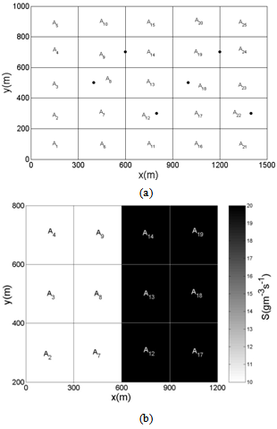Figure 1. (a) Sub-domains representation, in a 2D projection (x,y), with different emission rates, and black points (●) represent the sensor position at 10m height. (b) The gray-scale represents the emission rate

There are several methods to compute the regularization parameter (Section 3). Here, a numerical experimentation was employed. The value found was α=10^-6 for Experiment-1, and α=10^-5 for Experiment-2[9].

Results for Experiment-2 are presented in Table 4 and Figure 3. The error between the exact values and estimated by the inversions calculated by following form:

(15)

Table 3. The values of emission rate estimation, using the Q-N method, with the data from Experiment-1

In the Experiment-1, a global error around 2% is found from to inverse solution – see Table 3. For the region-1, the error in the estimation is 10%, and for region-2 the error is 3%. The biggest error estimation are verified for sub-domains A₉ and A₁₄, with error of 55% and 42%, respectively.

Table 4 shows the estimated emission rate for each sub-domain. The global estimation error enhances to 6.7%. The error for region-1 from the inverse analysis decreases to 1%, but the error for region-2 increases to 11%. The worse estimation is related to region-2, where the sub-domains A₁₂ and A₁₄ present approximately 6% of error.

Table 4. The values of emission rate estimation, using the Q-N method, with the data from Experiment-2

The error for the inverse solution for experiment-2 is greater than experiment-1, as expected, since the level of noise in the measured data is higher in experiment-2. The results suggest that the inversion approach is effective, and the entropy regularization of second order is also appropriated.

One feature to point out is the use of source-receptor strategy. Indeed, this scheme allows a reduction of the computational complexity to compute the forward problem. As the inverse analysis is formulated as a non-linear optimization problem, this implies an iterative process requiring to execute several (thousands) times the forward problem.

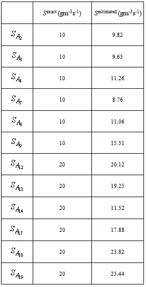
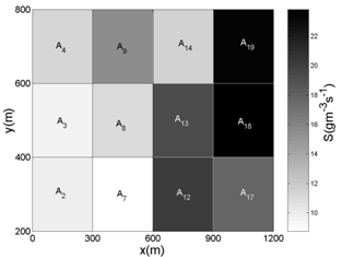Figure 2. Representation of the of emission rate estimation in the domain with data from Experiment-1

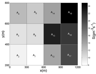Figure 3. Representation of the of emission rate estimation in the domain with data from Experiment-2

5. Conclusions

The methodology proposed for estimating the emission rate term and localization of the source/sink was effective to produce good estimations for pollutant emission rate with second order maximum entropy. Good results were obtained even for a high level of noise, showing that the inverse model is robust related to the noise in experimental data. The determination of the regularization parameter by L-curve allowed finding an appropriated value for regularization operator, following the procedure presented by Hansen[21]. The source-receptor scheme is employed in the inverse analysis, in order to reduce the computational effort.

Future works will include the application of the methodology to real gas fluxes with different types of soil covering. Further we will employ other entropic regularization operators[25], and different optimization schemes for the minimizing functional (1), using stochastic schemes and/or approaches from artificial intelligence (neural networks, or fuzzy systems).

ACKNOWLEDGEMENTS

The authors would like to thank to the Brazilians (CNPq, FAPESP) and Italian agencies for research financial support. The first author acknowledges CNPq-Brasil (Proc. 20.0046/04-7) for the sandwich doctorate fellowship in the ISAC-CNR, Turin – Italy.