1. Introduction

Dispersion of pollution plumes in the atmospheric boundary layer (ABL) has undergone a considerable evolution from its early classification scheme according to stability to more advanced models that are based on the Monin-Obukhov similarity theory. However, the complexity more or less turbulent of the phenomenon is still manifest in parameterizations that hide physical details in phenomenological coefficients and it would be desirable to shade further light on at least some of their properties. In this sense the current discussion is an attempt to identify significant contributions from first order perturbation theory with equivalent findings from a spectral theory approach.

Studies of pollutant dispersion, and in particular of its governing advection-diffusion equation (ADE), have a long tradition of being treated analytically. In fact analytical solutions are of fundamental importance in understanding and describing physical phenomena. Analytical solutions explicitly take into account all the parameters of a problem, so that their influence can reliably be investigated. It is also easy to obtain the asymptotic behaviour of the solution, which is usually more tedious to generate numerically.

Moreover, in the same spirit as the Gaussian solution (the first solution of the ADE with the wind and eddy diffusivity coefficients set constant in space), the former suggest the construction of operative analytic models. Gaussian models, so named because they are based on the Gaussian solution, are forced to represent real situations by means of empirical parameters, known as "sigmas". They are fast, simple, do not require complex meteorological input, and describe the diffusive transport in an Eulerian framework, making the use of measurements easy. For these reasons they are still widely employed for regulatory applications by environmental agencies all over the world in spite of their well-known intrinsic limits.

A significant number of works regarding the ADE analytical solution (mostly with a two-dimensional treatment) is available in the literature. Among them we mention the works[1-17]. However, above solutions are valid for very specialized situations: only for ground level sources, an ABL of infinite height, or specific vertical profiles for wind and eddy diffusivities.

Reference[18] presented an analytical solution, called ADMM (Advection Diffusion Multilayer Method) for a limited ABL height and general wind and eddy diffusivity vertical profiles, but expressed by a stepwise function (see[19] for a complete review). The ADMM method was further associated with the Generalized Integral Transform Technique (GITT) to obtain a three-dimensional solution [20-23]. Some of the above solutions were used[17] in operational air pollution models.

Finally, a general two-dimensional solution without any restrictions in the spatial function describing the wind and eddy diffusion coefficients was presented in[24-26]. The method used was the Generalized Integral Laplace Transform Technique (GILTT). That is an analytical series solution, including the solution of an associated Sturm-Liouville problem, the expansion of the pollutant concentration in a series in terms of the attained eigenfunction, replacement of this expansion in the ADE and, finally, taking of moments. This procedure leads to a set of differential ordinary equations that are analytically solved by Laplace transform technique. A complete review of the GILTT method is given in[27]. For the three-dimensional solution see[28-32].

All these analytical methods have in common the fact that three-dimensional, transient equations are not easy to treat. One way around this difficulty is to apply a first order perturbative analysis to the original problem before applying the transform technique. Recent meteorological literature contains a number of studies employing perturbation techniques, but none of them uses them to simplify the analysis via transform methods. In the literature some problems are obviously better suited for perturbation analysis due to the presence of a native small parameter, as is the case with the flow over smooth terrain (for example[33]). Regarding air pollution studies, however, very few results are found. An example is[34] that use singular perturbation techniques to obtain a new analytical solution to the 1-D transient convection-diffusion equation.

The present study uses a first order perturbation technique known as IVT (Intermediate Variable Technique, briefly reviewed in what follows) to simplify the three-dimensional advection-diffusion equation. Results are compared with preceding complete GILTT results to show that the neglected terms are indeed small.

2. Perturbation Techniques

The solution of regular problems by perturbation methods, although not always easy, is generally straightforward because the solution remains valid for the whole domain of interest. This is not the case with singular problems, thus a number of techniques were developed to deal with the mathematical difficulties arising. The most well-known are the Matched Asymptotic Expansions Technique, the Method of Multiple Scales and the Method of Strained Co-ordinates. In the analysis that follows we employ the Intermediate Variable Technique (IVT), which is less known, and thus is briefly reviewed.

The IVT has its roots on Matched Asymptotic Expansions. It is based on the ideas of[35] and can also be found in[36]. When matched asymptotic expansions are used to solve boundary layer problems, a special variable (called the intermediate variable) is used to match the inner and outer solutions (in case they are only two). This is achieved through a co-ordinate stretching (or rescaling) of the kind, where x is the independent variable, is the small parameter, a is (often but not necessarily) an integer and is the stretched co-ordinate. After substituting x by into the equations under study, a is allowed to vary and the resulting possibilities of matching are investigated. The values of a that gives such matching, shows where the boundary layers are, allowing for the construction of the inner and outer solutions that describe the whole domain of interest.

The IVT is a modification of this method and is indeed implicit in the search for afore mentioned boundary layers. In IVT, no inner or outer asymptotic solutions are sought. The intermediate variable is used to define the layers where different terms dominate in the original equation and in first order approximation. The exponent a is abandoned and is allowed to vary continuously in the interval ]0,1] in the expression . The method thus shows the relative importance of terms in the original equation as one move from the boundaries of the problem to the far field.

3. Mathematical Analysis

The time-dependent three dimensional Cartesian coordinates, advection-diffusion equations that describe the dispersion of a passive pollutant released by an elevated source on a statically neutral atmosphere are[37]:

(1)

(2)

(3)

in 0 < x < L_h, -B < y < B, -B < z < B, where all symbols have their usual meaning. Thus, bars over the variables represent time-averages and primes indicate turbulent fluctuations, c is the volumetric concentration of the passive contaminant (in units of g/m³ for example), , U = (u,v,w) is the wind velocity vector with Cartesian components in the directions x, y and z, respectively, ρ is the air density and νc is the molecular diffusivity. The terms represent the turbulent fluxes of contaminants, in the longitudinal, crosswind and vertical directions.

The source term is absent in eqn. (3) because it is included in the boundary conditions, which are

(4)

(5)

Here, Q is the emission rate at height of the source located at the origin, δ is the Dirac-delta function, B is the lateral dimension of the plume in both y and z directions, and L_h is its length.

To render eqns. (1) to (3) dimensionless, typical values for all variables must be chosen. We propose to use the geostrophic wind velocity, U_g, for the x and y mean wind velocity components u and v, and a characteristic velocity (to be determined later) W_c for the z component. We may use the friction velocity, , for all turbulent velocity components and the concentration at the source for the mean concentration. For the turbulent fluctuations of the concentration we assume to supply with an approximate estimate. Time may be rendered dimensionless using the characteristic response time of the ABL to surface forcings, t_c.

To cast the space variables in dimensionless form we recognize that the atmosphere and the plume have different length scales. Thus, for the atmosphere we shall use the characteristic horizontal PBL length, L_h, for x and y, and the characteristic vertical PBL length, L_v for z but for the plume we shall use L_h for x but we apply the characteristic plume width, B, for y and z. The resulting expressions for the dimensional space variables are, thus, X₁ = x/L_h, Y₁ = y/L_h, Z₁ = z/L_v, to be used in eqns. (1) and (2) and X₂ = x/L_h, Y₂ = y/B, Z₂ = z/B, to be used in eqn. (3). From these relations it follows that X₂ = X₁, Y₂ = Y₁L_h /B, Z₂ = Z₁L_v /B. Applying all the transformations to non-dimensional coordinates and the preceding three relations to eqns. (1) to (3) yields

(6)

(7)

(8)

in 0 < X₁ < 1, -1 < Y₁ < 1, -1 < Z₁ < 1, where uppercase letters represent non-dimensional variables and τ is the non-dimensional time.

Without loss of generality, the coordinate system of the problem can be rotated such that next to the surface. In this case, eqn. (6) implies that W_c must be such that L_hW_c/L_vU_g.= O(1), otherwise, ∂_X1U = 0 or ∂_Z1W = 0 if L_hW_c/L_vU_g.= o(1) or if o(L_hW_c/L_vU_g) = 1, respectively. The first possibility implies that there is no streamwise u velocity variation in the plume in first order approximation; the second that there is no vertical w velocity variation, respectively. Both conditions are known to be unreasonable, in the general case, for the PBL.

Due to the random nature of turbulent fluctuations, the coordinate system cannot be oriented such that and, therefore, the above conclusion does not apply to eqn. (7). In fact, for neutral atmosphere, (L_h/L_v) = O(1)[38] holds. Substituting this relation and L_hW_c/L_vU_g.= O(1) in eqns. (6) to (8) and for convenience introducing the small parameters ε_t, ε_*, ε_c*, ε_d results in

(9)

(10)

(11)

where ε_t = L_h/t_cU_g, ε_* = u_*/U_g, ε_c* = c_*/c_s, ε_d = ν_c/L_hU_g.

Typical values for the variables involved in the definitions above are t_c = 3,600 s ([37]), u_* = 0.3 m/s and U_g = 10 m/s[38], ν_c =10^-5 m²/s ([39]), L_h = L_v = 1 km[38], c_s = O(10^-7) kg/m³[40] and c_* = O(10^-8) kg/m³. The value adopted for L_v may vary in the case of a stratified atmosphere. The typical value for c_* was obtained through comparison with specific humidity values, i.e., supposing that c_*/ c_s = q_*/q_max, where q is the specific humidity, q_* = 5•10^-3 and q_max = 4•10^-2[37]. With the values listed above, the small parameters take the following typical values: ε_t = 2.8•10^-2, ε_* = 3.0•10^-2, ε_c* = 10^-1, ε_d = 1.4•10^-9. With those values, it is true that ε_d = o(ε_*ε_c*)², a relation that is going to be used later.

To stretch the lateral coordinates of the problem it is necessary to know where the boundary layers of the problem are. This is not possible, in general, without knowing the exact solution of the problem in advance or details of its physics. For the PBL, physics indicate that it is located next to the surface, thus we use

(12)

where ε ⊂ ]0,1]. For the plume, the general form of the equation suggests[41] that eqn. (3) contain two boundary layers at the extremes of its domain, i.e., at y = ±B and z = ±B. To stretch this kind of problem we use

(13)

again for ε ⊂ ]0,1]. Substituting eqns. (12) and (13) into eqns. (9) to (11) yields

(14)

(15)

(16)

Rotating again the coordinate system such that implies that the derivatives for and derivatives in eqn. (14) are of the same order, irrespective of the value of ε. Upon rotation it such that implies the and derivatives are of the same order and, thus, all terms in eqn. (14) are of the same order of magnitude. This implies that all the advective terms of eqn. (16) are of the same order of magnitude too. 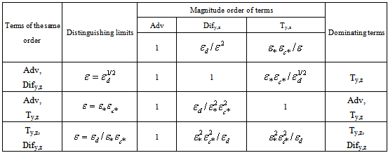Again, the coordinate system cannot be rotated such that or so that such a conclusion does not apply to eqn. (15). These conclusions allow us to write eqn. (16) in an order of magnitude fashion,

(17)

where 'Ac' stands for the accumulation effect, 'Adv' for the advection effect, 'Dif' for molecular diffusion and 'T' for turbulent diffusion. The subscripts stand for the direction of the derivative.

Table 1. Distinguishing limits

Now we proceed to calculate the distinguishing limits for eqn. (17), i.e., the values of ε for which its terms get the same order of magnitude. In general, this can be achieved comparing in principle all possible pairs of terms, but here we need not consider all pairs because some terms are always of smaller order than others as ε → 0, as for instance Dif_x and Dif_y. The following table shows the result of the comparison.

In spite of the appearances, only two distinguishing limits result from the analysis: ε = ε_*ε_c*, where Adv = O(T_y,z), and ε = ε_d/ε_*ε_c*, and Dif_z = O(T_y,z). The value of ε for Adv = O(Dif_z) does not constitute a limit because it is dominated by the T_y,z term in this case.

If we allow ε to vary between the two obtained distinguishing limits, domination of only one term in eqn. (17) results. For example, in the region where ε_d/ε_*ε_c* << ε << ε_*ε_c*, only T_y,z dominates. Returning the T_y,z type symbols to their dimensional form the resulting first order equations and the respective regions of validity are

(18)

(19)

(20)

(21)

(22)

The expressions defining the regions of validity in terms of y where obtained noting that in the stretching process we make use of

(23)

and thus

(24)

and similarly for z. Figure 1 depicts the dominant terms yielded by the analysis. The regions are not drawn as to represent realistic scale ratios.

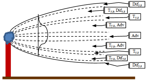Figure 1. Schematic drawing of the pollutant plume, showing regions of dominance of the terms in equation (3)

4. The GILTT Method

The ADE of air pollution in the atmosphere, eqn. (3), is essentially a statement of conservation of the suspended material and it can be written as[43]:

(25)

where is the mean wind and S is the source term.

Equation (25) has four unknown variables (the concentration and turbulent fluxes) which lead us to the well known turbulence closure problem. One of the most widely used closures for eqn. (25), is based on the gradient transport hypothesis (also called K-theory) which, in analogy with Fick’s law of molecular diffusion, assumes that turbulence causes a net movement of material following the negative gradient of material concentration at a rate which is proportional to the magnitude of the gradient[42]:

(26)

Here, the eddy diffusivity matrix K = diag(K_x, K_y, K_z) is a diagonal matrix with the Cartesian components in the x, y and z directions, respectively. In the first order closure all information of turbulence complexity is contained in the eddy diffusivity.

Equation (26), combined with the continuity equation of mass, leads to the ADE[43]:

(27)

The simplicity of the K-theory of turbulent diffusion has led to the widespread use of this theory as a mathematical basis for simulating pollutant dispersion (open country, urban, photochemical pollution, etc.), but K-closure has its known limits. In contrast to molecular diffusion, turbulent diffusion is scale-dependent. This means that the rate of diffusion of a cloud of material generally depends on the cloud dimension and the intensity of turbulence. As the cloud grows, larger eddies are incorporated in the expansion process, so that a progressively larger fraction of turbulent kinetic energy is available for the cloud expansion.

Equation (27) is considered valid in the domain (x, y, z) ϵ bounded by 0 < x < L_x, 0 < y < L_y and 0 < z < h and subject to the following boundary and initial conditions,

(28)

Instead of specifying the source term as an inhomogeneity of the partial differential equation, we consider a point source located at an edge of the domain, so that the source position r_S = (0, y₀, H_S) is located at the boundary of the domain r_S ϵ . Note, that in cases where the source is located in the domain, one still may divide the whole domain in sub-domains, where the source lies on the boundary of the sub-domains which can be solved for each sub-domain separately. Moreover, a set of different sources may be implemented as a superposition of independent problems. Since the source term location is on the boundary, in the domain this term is zero everywhere (S(r) 0 for r ), so that the source influence may be cast in form of a condition, where we assume that our coordinate system is oriented such that the x-axis is aligned with the mean wind direction. Since the flow crosses the plane perpendicular to the propagation (here the y-z-plane) the source condition reads:

(29)

where Q is the emission rate (in units of g/s), h the height of the ABL (in units of m), H_S the height of the source (in units of m), L_x and L_y are the horizontal domain limits (in units of m) and represents the Cartesian Dirac delta functional.

In order to solve the problem (27) we reduce the dimensionality by one and thus cast the problem into a form already solved in[27]. To this end we apply the integral transform technique in the y variable, and expand the pollutant concentration as:

(30)

where R = (R₁, R₂, . . .)^T and Y = (Y₁,Y₂, . . .)^T is a vector in the space of orthogonal eigenfunctions, given by with eigenvalues for m = 0, 1, 2, … . After substitution of eqn. (30) in eqn. (27) and taking moments, we obtain a set of M + 1 two-dimensional diffusion equations:

(31)

Observe that to obtain eqn. (31) we specialized the application for a pollutant dispersion problem in PBL, assuming that the speeds and takes the null value. We neglect the diffusion component K_x because we assume that the advection is dominant in the x-direction, i.e., . We also consider that K_y has only dependence on the z-direction.

Problem (31) is solved using Laplace transform technique and diagonalization, following the works[27][29][30].

The specific form of the eddy diffusivity determines now whether the problem (31) is a linear or non-linear one. In the linear case the K is assumed to be independent of , whereas in more realistic cases, even if stationary, K may depend on the contaminant concentration and thus renders the problem non-linear. However, until now no specific law is known that links the eddy diffusivity to the concentration so that we hide this dependence using a phenomenological motivated expression for K which leaves us with a partial differential equation system in linear form, although the original phenomenon is non-linear. In[32], an example demonstrates the closed form procedure for a problem with explicit time dependence, which is novel in the literature.

4. Discussion

The reliability of each model strongly depends on the way turbulent parameters are calculated and related to the current understanding of the PBL. Following[44], during convective conditions at the following relation is used:

(32)

On the other hand, in our simulations, we use the wind speed profiles described by a power law, according to[45],

(33)

where u_z and u₁ are the mean wind velocity respectively at the heights z and z₁, while n is an exponent that is related to the intensity of turbulence[46]. The value used for convective conditions is 0.1).

As an example, we used a boundary layer height of 1000m, source height of 500m, friction velocity of 0.3m/s, distance from the source of 200 m.

In the further we compare the solution of the ADE to the dominant contributions from perturbation analysis. To this end we amplify or suppress certain characteristics, i.e. diffusion, advection, turbulence, and show the results in figures 2-4.

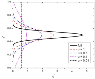
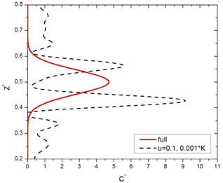
Figure 2. Full solution of the ADE and advective dominance

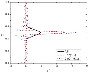
Figure 3. Full solution of the ADE and turbulence dominance

In the limit ν_c → 0 molecular diffusion is faded out, which is usually disregarded in dispersion models. A comparison of the inclusion or omission of molecular diffusion shows no visible difference. Upon reducing diffusive and dissipative contributions maintains the advective dominance, which is shown in figure 2. The solid line corresponds to the full solution, whereas the dotted and dashed lines represent the reduced solutions. The oscillatory character is clearly a consequence of the approach and shows that in this limit the auxiliary problem is not the best choice to model the solution, because there is need for a higher dimensional functional space. Upon amplification of the turbulent effect one observes for small mean wind velocities the power of turbulence to effectively mix the pollutant with the carrier (the air). Further the presence of the remaining contributions restricts the spread of pollutant into a narrow range in the stationary limit. The last analysis (see figure 4) shows that, if there were a dominant molecular diffusion, a larger spread and more pronounced fluctuations were the result. From a comparison of possible values for the concentrations shows that the presence of advection, turbulent and dissipative mechanisms suppress effects due to molecular diffusion. The three analysed limits show the potential, that using findings from perturbation analysis may help identify the physical profile of the plume.

Figure 4. Full solution of the ADE and molecular diffusion dominance

5. Conclusions

With the present discussion we presented a first attempt to disentangle relevant physical mechanisms that constitute the dynamics of pollutant dispersion in form of plumes. Although there are fundamental differences in the two approaches, one based on an order of magnitude analysis, i.e. small parameter expansion, the other constructed from spectral theory resulting in a solution that makes use of a parameterized turbulence model in form of phenomenological eddy diffusivity.

More specifically the turbulent pollutant flow in IVT results from a perturbation order evaluation that substitutes the otherwise necessary closure, such as Fick's law among other possibilities. Therefore turbulence closure is local due to the consideration of first order terms only.

The advection diffusion equation approach with its space time dependent eddy diffusivity function represents turbulent properties and is not restricted to a special regime, i.e. it is globally valid.

Thus, although based on different footings, the IVT approach supplies with a qualitative hierarchy of mechanisms, that together with the spectral theory based approach allows to turn these findings semi-quantitative by fading out higher order to leading order terms in the ADE solution.

The combination of IVT and GILTT provide a first step that allows to tag the mechanism profile or equivalently the dynamical profile of pollution dispersion in plumes. In future investigations we will focus on the dynamical equation for pollutant dispersion fluctuations (higher statistical moments) in order to allow for comparisons between the "local closure" from the perturbation analysis and specific limits of advection-diffusion variance. Such a procedure will open pathways to analyse compatibility of perturbative local closure with global eddy diffusivity parameterization.

ACKNOWLEDGEMENTS

The authors wish to thank CNPq (Conselho Nacional de Desenvolvimento Científico e Tecnológico), FAPERGS (Fundação de Amparo à Pesquisa do Estado do Rio Grande do Sul) and FAPEMIG (Fundação de Amparo à Pesquisa do Estado de Minas Gerais) for the partial financial support to this work.