1. Introduction

Pantanal is one of the main biomes in South America, being the biggest flood plains on Earth and characterized by alternating flooded and dry regions. It extends through the States of Mato Grosso and Mato Grosso do Sul, from the brazilian side, through Bolivia at east and through Paraguai at north. It is located at the South America central region (between 16º e 21º de latitude south and 55º to 58º longitude west).

Its vegetation is characterized by savanna steppe, that means, a vegetation with predominance of grass, few trees and a relatively plain terrain, with low elevation in relation to sea level (around 100m)[1].

The spatially and temporally irregular occurrence of flooding in Pantanal's savanna differentiates its flora and fauna from other regions. Such irregularity generates peculiar variability patterns of micrometeorological variables for each season, with frequent fire in dry season and irregular flooding during the wet period, in which local farmers are forced to reallocate hundreds of cattle to higher regions[2]. Such peculiarity associated with the passage, through Pantanal, of moisture coming from the Amazon to the south of South America (SA) makes this ecosystem an interesting source of research[3]. The passage of moisture from Amazon to south SA has already been well documented[3].

The reference[3] relates results from the (South American Low-Level Jet Experiment) experiment, taken place at SA, which describes the continental troposphere flow and its relation to moisture transport from the Amazon to the southeast SA. Pantanal's moisture regime is directly influenciated by (South American Low-Level Jet –), which interact with river Plate’s Basin. Such interaction allows the modification of the region's precipitation regime, whether the season is dry or flooded, and makes Pantanal a differentiated ecosystem from forest regions, such as Atlantic forest and Amazonia. Despite these characteristics, few micrometeorological studies have been made on this region[2].

The Interdisciplinary Pantanal Experiment (IPE-1) was the first fieldwork accomplished to characterize the Atmospheric Superficial Layer (ASL) on Pantanal, implemented between May and June 1998. A preparatory pre-campaign was realized in 1996, involving a portable tower, experimental campaign IPE-0. Other two experimental campaigns occurred, aiming a better characterization of the regional micrometeorological parameters: IPE-2, in September 1999, when the experimental site was dry, and IPE-3, in February 2002, when the experimental site was flooded.

In recent published articles[4,5], Low-Level Jets () possible actions upon intermittent turbulence formation[1] and upon variance and covariance of turbulent variables[2] at the Nocturnal Boundary-layer (NBL) were discussed. In reference[4], three turbulence regimes at NBL above the USA central region during the Cooperative Atmosphere-Surface Exchange Study (CASES-99) experiment are proposed: regime 1, in which turbulence is weak with a mean wind velocity value below a threshold value (V_t); regime 2, characterized by a strong turbulence when mean wind velocity is higher than the threshold value (V_t); and finally regime 3, which presents moderate-intensity turbulence, marked by sporadic bursts due to type “top-down” mix mechanisms. These turbulence regimes are highly influenciated by the presence of . Without such presence, regime 1 prevails[1]; regime 2 occurs when is strong enough to increase wind velocity above the threshold value V_t; regime 3 finally occurs when wind shear below is strong enough to generate shear instability propagated in a descendent way, downward.

From another perspective, reference[5] discusses shear-sheltering mechanism. Shear-sheltering mechanism generated by a would function as a barrier to the descendent propagation of the jet action to the surface.

In another words, in the last reference, would perform low-frequency turbulent energy suppression, in the wind velocity components spectra, due to an increase of wind shear in the layer below the . In[5] evidences of shear-sheltering were not found. The expected decrease in contributions to length scales above high was also not found. Considerable increase of energy contributions to length scales below scales were observed, as well as to scales above the jet height, where a decrease was expected. Considering that the shear-sheltering theory may be applied to , the authors attribute the absence of this shield mechanism in an experimental site in the North American state of Kansas to the vortex characteristics there and formulate the hypothesis that, under distinct experimental conditions, the shear-sheltering theory may be detectable.

actions were recently studied to various experimental sites and in many different perspectives[6-23]. In this context, the present paper presents an aspect not yet analyzed about the action of in NBL. Applied to the context of an experimental site in Pantanal, this work aims to describe the modification of action in scale of the different kinds of in the regional NBL through time. Besides, the influence of the surface condition modification in this action was observed. Such surface alteration is due to the seasonal change in the region (dry and flooded sites). The focus of the study lays upon the wind vertical velocities variances (w) and potential temperature (θ), as well as upon the covariance between these two variables, projected in scale, to evaluate the possibility to apply the shear-sheltering mechanism described in[5] at the Pantanal region.

This research performed 6 case studies. For each season (dry and flooded) the following situations were studied: a) -absent; b) with weak shear (-WS)[17]; and c) with strong shear (-SS)[16]. Contributions to the eddy covariance wθ at length scales larger than the JBN height have been detected as positive contributions to the sensible heat flux. Another interesting finding was the evolution of a action which has generated top-down mixing, as described in references[4, 16]. It was noticed that such an event increased the available energy to w through time in different scales. Next section describes the experimental site and data used in the present paper.

2. Experimental Site and Data

Experimental data were obtained during the IPE-2 and IPE-3 campaigns, related to Pantanal dry and flooded seasons, respectively. The IPE-2 was accomplished during the period from 07 to 22 September 1999. The IPE-3 was accomplished during the period from 16 to 28 February 2002. Both campaigns took place in an experimental site located at southeastern Pantanal (19º34’S, 57º01’W), near the city of Corumbá, near the Miranda River, at the Brazilian state of Mato Grosso do Sul[1].

At the experimental site, wind is mainly northwesterly orientated. Due to South America Low-Level Jet interaction, moisture transported by it from the Amazon, the Andes Cordillera deflects such system to the south of South America[3]. Such interaction is one of the factors which allows a differentiated behavior in the regions hydrologic cycle[24]. This cycle has its behavior characterized by inter-annual Pantanal terrain overflow oscillation and great precipitation occurrence during summer (80% between November and March)[25]. Vegetation is characterized as “cerrado”. At east there is gramineae predominated. At north and west one observes an irregular and sporadic disposal of medium-size trees (median size of 10m) along with bushes and creepers. At south, a large riparian and paratudal area can be found[1].

Data used in this work were obtained through radiosonde, anemometer and sonic thermometer. Radiosonde data were collected by a Väisälä RS80 model, for both campaigns. In IPE-2, 55 radiosonde in different hours were taken. From the total collected, 20 radiosonde occurred during the night-time period. This work's night-time period denomination followed the classification established by the references [26,27]. For IPE-3, 80 radiosonde in different hours were taken, 32 of them occurred during the night-time period. The total of 52 night-time period radiosonde, in both campaigns, cannot be analysed in order to detect the presence of , being then analyzed an amount of 29 radiosonde to both campaigns (11 to IPE-2 and 18 to IPE-3). Problems found in radiosonde were: a) lack of wind intensity and direction (19 events) and b) signal loss (4 events).

Fast response data were recorded by an anemometer and sonic thermometer (model 3D CSA-T3 Campbell), for the following wind velocity components: longitudinal (u), transversal (v), vertical (w) and for temperature (T). Sampling rates were 16Hz to IPE-2 and 8Hz to IPE-3, collected from the top of a micrometeorological tower, at 25m high.

Data quality control procedures were based in the methodology proposed by reference[28]. From the total of 29 days of fast response data, about 34% of it had to be discarded (the equivalent of 10 days). Data file discarded in posterior analyses were due to: a) damaged files; b) gaps in standard files for each season; c) excess of spikes. After initial data processing, cross-checking involving radiosonde results and fast response data was performed, generating six one-hour rapid-response data intervals for case study. Beyond detection, radiosonde data were used to classify as: a) Weak Shear and b) Strong Shear, according to criteria established in reference[17]. Next section will describe in details the applied criteria and treatment applied in case studies.

3. Theoretical Elements and Methodology

It will be seen next how radiosonde were used in detection and classification, some important aspects of Wavelet Transform and its application to fast response data analyses, interval definition criteria used in case studies and, at last, the methodology applied in case studies under action of in Pantanal's NBL.

3.1. Low-Level Jets Detection and Classification

Radiosonde data were used to characterize presence. Its identification is made through wind velocity profile. A is characterized by a maximum peak in vertical profile in wind velocity with a difference of 2ms^-1 above and below this maximum[29]. Other authors establish different restrictions to this definition, for example: maximum velocity must be present in the first kilometer above surface[19] and the difference of 2ms^-1 must be established in a difference in height of 200m[6]. Reference[16] was one of the first authors to highlight a 's ability to, once established above surface, generate jet mixing downwards in such a way to cause modification in thermodynamic structure below and take instability to surface.

Reference[18] related an experience which simulates a CLN in a wind tunnel with . It is then observed a turbulence “bursting” in a lower portion of the boundary layer, occurrence also related in other works[20,21]. In[10] related the presence of a produces a great vertical wind shear, producing upside-down mechanical turbulence. This causes a mixing strong enough to allow estimations to momentum and sensible heat flux, based on the Similarity Theory (ST) to be in perfect agreement with experimental data. However, in certain conditions, may not generate significant mixing, that is, a classification must be made. Two of them are defined as: a) the one which does not cause upside-down mixing (-WS) (Figure 1-a) and b) the one which causes upside-down mixing (Mixture ) (Figure 1-b). -WS classification adopted in this work is the one proposed by[17].

Reference[15] has discussed the influence of the presence in a CO₂ night change in a forest in Florida, USA. This research related the action with atmospheric stability, velocity, friction and Turbulent Kinetic Energy (TKE) variation. They describe action as a forcing which causes variation in atmospheric stability through increase of friction velocity. This would increase CO₂ and TKE change between surface and atmosphere due to an increase in the vertical wind velocity, w, variability. References[8,9] present a vertical distribution in TKE through the vertical velocity variance (σ²_w) associated to LLJ. It was found there that the TKE vertical distribution relates directly to a Gradient Richardson Number profile (Ri). To less stable profiles, TKE has its maximum at the surface and decreases with height until the center. To higher stable profiles, TKE has its maximum near the center. In[21] used Wavelets Transform (WT) to demonstrate that strong eddies, which interact with the turbulence scales of the forest top, contribute to the counter-gradient scalar flux production. These contributions are present in the variance spectrum and cospectrum obtained via WT. Spatial scales of these large eddies are greater than height. These upside-down structures are responsible for the increase in wind velocity components variance and momentum and scalar flux.

In[17,21] the authors discuss the ideal conditions of manifestation of a that does not generate upside down mixing. Reference[14] concludes that this kind of is characterized by accumulation of CO₂ gas below velocity maximum. Some of the ideal conditions established by them were: a) a minimum of wind velocity unbounded from the surface; b) this maximum must de located in the region below temperature inversion, which maintains a concentration of gas due to the strong gradient of temperature above. This way, has the possibility to promote coupling between surface-atmosphere, that is, causing upside-down mixing or promoting surface shielding, once the mixture forced by the is not able to overcome thermal inversion, respectively.

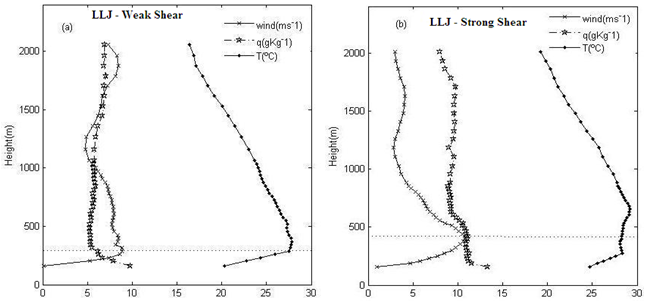Figure 1. Example of detection and classification. (a) to a – Weak Shear at 18 September 1999 at 0200, local time. (b) to a Strong Shear at 19 September 1999 at 0200, local time

Therefore, in this work were identified and classified, where two types of them were defined: a) those which do not generate top-down mixing (-WS) and b) those which do cause top-down mixing (-SS), according to the methodology described above. Specific humidity profiles and potential temperature were used in order to differentiate types of . Specific humidity profile was used to characterize accumulation of gas below . -WS presents a decreasing gas profile until the maximum point in wind velocity profile. From this maximum's height, an increase in gas mixture with height is observed. Potential temperature profile to -WS has a thermal inversion up to a height which matches maximum velocity or exceeds it (figure 1-a). -SS may appear under a thermal inversion; however, its height does not exceed or it is coincident to the center (figure 1-b). Based on classifications established by[26,27], the night-time period is defined as the time interval between 2000 and 0600 (Local Time). All fast response data were submitted to WT, with Morlet as Complex Mother-Wavelet. Its choice is due to a its good resolution in the frequency[30-33].

3.2. Wavelet Transform

Wavelet Transform consists in localization (time or space) and scale decomposition of a temporal or spatial data series[31]. Such decomposition allows to split a data set in a group of scales under all locations in the series[32]. Decomposition occurs through inner product of the time-series and the wavelets. Wavelets are functions with the same form of a original function, the mother-wavelet. Wavelets are generated through mother-wavelet dilatation and translation, which holds the general form:

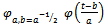(1)

Being “a” the dilatation parameter and “b” the translation parameter of the mother-wavelet. Parameter a^-1/2 holds the wavelet translated and dilated energy equals to that of the mother-wavelet. Increasing parameter “a” corresponds to a faster oscillation in the wavelet compared to the mother-wavelet (characterizing a high frequency oscillation). Decreasing parameter “a” produces a slower oscillation in the wavelet compared to the mother-wavelet (characterizing a low frequency oscillation). Parameter “b” modifies position, in the data series, of the wavelet center[33].

A mother-wavelet must satisfy the condition of admissibility, which consists in a fast decay to zero in the location and scale domain of the wavelet function, and it assures that the wavelet has a zero mean. Wavelet transform consists on:

(2)

being (*) the wavelet complex conjugate. Results of decomposition are the coefficients W_a,b, resulting from the inner product between the signal x(t) and wavelets φ_a,b(t).

3.3. Criteria Used to Choose the Investigation Time Periods

By defining the time in which presence of was detected and its respective classification, 6 intervals of 1 hour each have been selected in order to accomplish the case study. To avoid effects due to the Early Evening transition[34], as criteria to select the analyzed intervals, were adopted its greater possible distance from the transition period, the beginning of the temporal series middle in the mark of 30 minutes before the radiosonde launch, and the end of the temporal series 30 minutes after the radiosonde launch. This way, 1 hour of data associated to an occurrence event was available. This procedure was adopted based on what was observed in reference[16], where it is discussed the non-stationary top-down mixing characteristic caused by the jet, pointing out that sometimes these mixing effects are observed at the surface. It is expected that, through analysis via WT of such temporal series, it may be possible to extract relevant information about shielding or mixing processes temporal evolution associated to observed in Pantanal, during dry (IPE-2) and flooded (IPE-3) seasons. In order to accomplish a direct comparison among the scales where the studied parameters were projected and the scale associated to height[5], temporal scales were converted to spatial scales using Taylor's Hypothesis[35]. Based on the above criteria, the following time intervals were selected to be analysed, in Local Time (LT):

Table 1. Time Intervals selected to case studies

3.4. Case Studies

Using classification, a methodology similar to that on reference[35] was implemented to scale analysis of turbulent parameters associated to each one of the types, as well as to situations without , in both seasons. Thus w and θ variances and covariances between w and θ were calculated, being all projected in scale. A 5 minutes mean window was used for by scale calculations of turbulent parameters described above. This choice was a consequence of data being related to night-time situations. As described in reference[36], for night conditions, 5 minutes means capture all turbulent eddies contributions for NBL, for most of the time. For each 5 minutes intervals in the periods presented in Table 1,the described parameters were calculated. So, 12 curves to each one hour period were obtained, related to both seasons and to each classification related to presence and type. From this methodology, temporal evolution of analysed parameters can be evaluated, and how they modify in scale and time during the Pantanal dry and flooded season. Next, the obtained results are presented according to the methodology above described.

4. Results

This section will investigate the turbulent scale structure and its temporal variability in the Pantanal's NBL under LLJ's action, emphasizing the energetic distribution and sensible heat exchange to dry season (on which sensible heat flux are always negative) and for the flooded season (where there are many situations when heat flux are positive).

4.1. Low-Level Jets Actions in Energy Distribution in Specific Scales

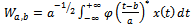
In the following figures some parameters will be presented, calculated in specific scales for the six time intervals described in Table 1: a) two intervals without ; b)two intervals with -WS and c) two intervals with -SS. In figures 2 to 4, the two intervals without are: a) the period between 0130 to 0230, in the night between 16 and 17 September 1999 (IPE-2, in Pantanal's dry season) and b) the period between 2300 and 0000, in the night between 17 and 18 February 2002 (IPE-3, during Pantanal's flooded season). The two intervals with -WS are: c) the period between 0130 and 0230, in the night between 17 and 18 September 1999 and d) the period between 0130 and 0230, in the night between 22 and 22 February 2002. At last, the two intervals with -SS are: e) the period between 0130 and 0230, in the night between 18 and 19 September 1999 and f) the period between 2300 and 0000, in the night between 18 and 19 February 2002. In the following section, actions of types of in w variances obtained in specific scales will be observed, related to the time intervals above described.

4.1.1. Intensification and Spectral Peak Shift Induced by Low-Level Jets

Figure 2 shows wind vertical velocity (w) variances on specific scales calculated in time intervals of 5 minutes, inside the obtained periods quoted above. It can be noticed that during the dry season (figures 2-a, 2-c and 2-e), the energy is mainly concentrated in length scales smaller than 75m, for situations with -WS and without , in all the analyzed time. Exception to this fact is observed in the -SS situation (figure 2-e), in which it is observed that, in schedule before detection (0200LT), energy concentrates on scales next to 1500m. Variance peaks distribution before detection hold values lower than the ones found near the 0200 schedule, when radiosonde was launched.

It is noticed that the w variance peak location (σ²_w) has its scale shifted to lower values in periods near detection time. Based on what is proposed by[16] about evolution, which produces top-down mixing, it is expected that, when a temporal series of a period of time associated to a jet occurrence is analyzed, a remarkable variance occurs in the most energetic scales associated to the turbulent kinetic energy or, in particular, w variance. The above result showed to be the expected from what was previously discussed.

By analyzing σ²_w results, obtained by WT application, it can be concluded that effectively remarkable shifts were found in scales corresponding to the maximum w variance (such variance calculated to successive 5 minutes intervals, as previously exposed). A 5 minute interval may be questioned as not ideal to calculate variance, but, as explained by[37], in its study about non-stationariety categorization of night-time turbulent time series, such calculations provide important information about non-stationarity of turbulent time series, independently of the statistical sense the parameter σ²_w must be associated to.

Along with this peak location shift, there is a considerable rise of the energy associated to this energetic peak. Energy reaches its maximum value in the interval between 0215 and 0220. After reaching its maximum peak, w variance presents a small oscillation in the energy present in the peak. Such behavior may be associated to the top-down mechanism acting in processes typically non-stationary observed on the surface as described in[16]. In item 4.3 there will be presented elements which effectively confirm such assumption.

Upside-down mixture action generated by probably reaches surface in a specific time, producing rise in turbulent energy at all scales below the one associated with height. This way, in schedule before action, a more stable stratification inhibits turbulent energy generation and concentrates energy in usually small scales, indicated by the buoyancy length scale (associated to the greatest turbulent eddy sizes), which present low values. With action and its expected action upon to the surface, it is observed a rise in mixing and energy available in scales below the one corresponding to the height, which amplifies the turbulent spectrum and its energy for several scales, specially below the scale associated to the height (indicated by a black arrow).

Differently from observation in dry season, situation with -SS in flooded season (figure 2-f), in length scales below 75m already holds a considerable amount of energy before detection schedule (2330LT). Such difference must be associated to the flooded Pantanal's differentiated behavior in night period, as discussed on[38], on which flooded Pantanal's NBL is more turbulent than NBL in dry period. This difference is possibly associated to the mechanism described by[39,40], in which water body causes heat absorption during the day and acts as heat source during the night. Therefore, flooded Pantanal shows such characteristics, allowing this observed energy distribution in small length scales.

-SS action during flooded season is observed through increase of energy associated to the w spectral peak. It is observed that, when close to the detection schedule (2330LT), w spectral peak holds energy higher to the values observed in the beginning of the case study involving -SS for the Pantanal's flooded season (2300LT). Thus, possibly acted intensifying energy in the scales below the one related to the jets' height. Next it will be discussed action in Pantanal's NBL under shear-sheltering mechanism.

4.1.2. The Shear-Sheltering Mechanism

The w variance in different schedules related to the -WS situation has considerable contribution for length scales above the height value (figures 2-c and 2-d). However, for the -SS (figures 2-e and 2-f), it is observed a decrease of energetic contributions on length scales located above the scale, except the detection occurred between 0200 and 0205, when a little increase of 1500m in length scale variance is noticed.

These results confirm some of the difficulties reported in observing the mechanism of shear-sheltering described by[5,20]. However, this case study result presents an indicative of the occurrence of -SS shear-sheltering in the dry season. Thus, it can be concluded that great eddies overcome shear region's height generated by and reached the surface in dry season, in the case of a -SS. According to the classification presented in[17], -WS does not produce shear with magnitude enough to reach the surface. A contrary effect is observable for the -SS, that is, -SS causes a strong shear which reaches surface and inhibits top-down eddies propagation on scales greater than that of the height, as is possible to observe in figures (2-d and 2-f). For -SS, the strong shear generated by blocked the passage of greater eddies at scales higher than the height[5,16,20,21]. Effectively this means that there occurs a process of filtering of the greatest eddies, associated with the highest scales observed at surface. This way, height imposes a superior limit to the greatest eddies' size in such a way that a energetic spectral band confined below the jet’s height scale presents.

At the flooded season (figures 2-b,2-d and 2-f) the presence of considerable energy peaks in height scales above 75m are observed, specially in situations without (figure 2-b). These peaks must be associated to the passage of a Gravity Wave (GW) in the period between 2305 and 2325 in the night between 17 and 18 February 2002. Length scales associated to GW observed in figures 2-b and 2-d are indicated by red arrows. After the GW event observed in the figure 2-b, it is noticed that the energy peak between 75m and 350m scale gradatively decreases its associated variances in such a way that the spectrum as a whole presents energy reduction, in all observed scales. In[42], in their study about GW in NBL it is reported a similar process. Pressure gradient relaxation effects established by the wave passage, as described in reference[42], as may be responsible for the delay in these spectral peaks decay observed here. To w variances in situation with , during the flooded season (figures 2-d and 2-f), a similar behavior as compared with the dry season is noticed, -WS presents peaks in length scales around 1500m, mainly detectable between 0210 and 0215. However, this behavior must be associated to the event of passage of an GW observed between 0210 and 0220 at the night of 21 to 22 February 2002. For -SS, a almost lack of existence of contributions to the w variance in scales above height can be noticed. This result reinforce what was discussed before for the dry season. This way, remarkable indicatives of the action of the shear-sheltering mechanism in Pantanal's NBL to both seasons (dry and flooded) are noticed.

Next it will be discussed the effect of modification of the surface conditions over variance of potential temperature (θ).

4.1.3. Effect of Modification of Surface Roughness Condition over Potential Temperature Variance

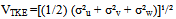
Figure 3 presents T variances in specific scales for 6 time series identified at item 3.3. To the flooded season (figures 3-b,3-d and 3-f), it is observed that the main contributions to T variance, in all schedules and in all three situations (-absent, -SS and -WS) are relative to length scales above1500m.

This result may be associated to low-frequency flow patterns generated by different water bodies present in Pantanal[41]. These low-frequency peaks come from the manifestation of the existence of an unstable layer next to the water level surface, once local circulations in multiple scales may emerge due to temperature horizontal gradients present between multiple dimension lake surfaces, located in flooded Pantanal, and non-flooded regions, both interacting with atmosphere[39,43,44]. Actions of these different gradients are expressed as these T variance peaks in the low frequency spectral band.

It must be highlighted the considerable landscape alteration observed in the Pantanal during flooding. In flooded season, it occurs the formation of many small shallow lakes, whose dimension and depth alterates along the season. It is true that they present multiple dimensions, though is not known from article in literature that statistically approaches its distribution. However, experimental sites located in landscapes where exists lakes with several dimensions had already been object of study[40]. As the authors say, the properties of these lakes differ from those of the surrounding terrain, as in the albedo case (usually smaller) and superficial roughness (which decreases above the water masses), with notable consequences to generation of local circulations.

Beyond these physically relevant aspects, others were also highlighted in study of reference[40], regarding the peculiarities of surface energy balance in such conditions. In addition to water having a high heat capacity, energy exchange between lake surface and its deeper water layers is more effective than that between the surface and deeper soil layers. By the way,[1] presented results of numeric simulation about the importance of heat storage by mass of superficial water of Mato Grossense Pantanal during the transition period from the humid to the dry season (experiment IPE-1).

For the dry season (figures 3-a,3-c and 3-e), considerable contributions in small length scales, around 75m, are noticed. Such result may be consequence of the difference of surface roughness between dry and flooded season. The smallest surface roughness caused by the existence of a water layer, in the flooded season, possibly inhibited the presence of energy peaks for T variance in smaller length scales[41]. That is, results seen to reflect the horizontal heterogeneity in mechanical and thermal roughness elements, in addition to present contributions, both mechanical forcing and buoyancy, to generate turbulent kinetic energy and temperature variance[39,40,43,44].

For -WS situations (figure 3-c), in dry season, a decrease in contributions to T variance in length scales below height and an increase in contributions to variance in scales above height, after jet detection time, is observed. This behavior must be associated to the action of top-down mechanisms, as discussed in[4]. Item 4.3 will present new elements to confirm such assumption.

For -SS situations (figure 3-e), the opposite process happens, that is, contributions to scales smaller than jet’s height increase and contributions on scales above height in variance of T decreases. Such rise is due to the mixing process caused by below its center[4,16].

In the next section, action on sensible heat flux by Pantanal NBL scale to dry and flooded season will be investigated.

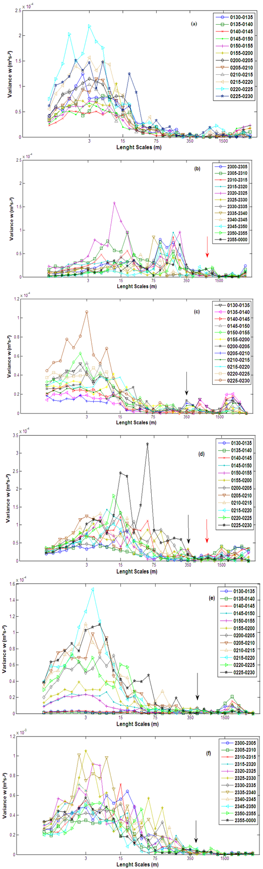Figure 2. Temporal evolution of vertical velocity variance (w) in scale, to: (a) and (b) without presence, (c) and (d) to a -WS and (e) and (f) a -SS. Figures (a), (c) and (e) are related to the dry season and figures (b),(d) and (f) to the flooded season, respectively. The black arrow indicates scale associated to height and the red arrow indicates scale associated to a Gravity Wave event

4.2. Action of Low-Level Jets in Sensible Heat Exchange

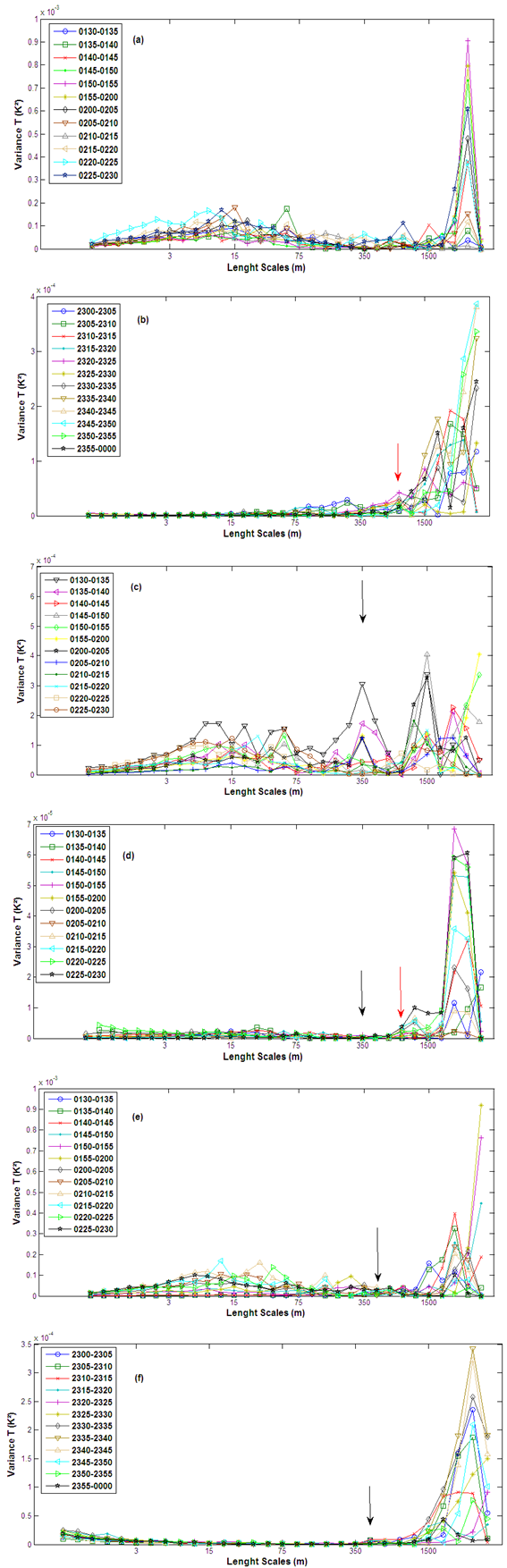
In order to analyze the influence of action upon different scales in sensible heat flux, covariance between w and T, in scale, was calculated, according the methodology presented in[35].

Figure 4 present covariances between w and T, by scale, for the periods described in methodology (section 3). Important differences between the two seasons are observed. In dry season (figures 4-a,4-c and 4-e), negative contributions to sensitive heat flux predominates. In flooded season (figures 4-b,4-d and 4-f), initially in -ABSENT situation, positive contributions to heat flux predominate. Such contributions must be consequences of the heat source existence during the Pantanal night-time period. As night goes by, water reduces its contribution to heat flux due to heat loss to the atmosphere, with consequent fall of lake surface temperature until it becomes lower than atmosphere's temperature. At the end of this period, negative contributions to sensible heat flux can be observed.

-SS, in dry season (figure 4-e) causes gradatively decrease of positive contributions for the sensible heat flux in scales above 1500m. At the end of the period, these scales begin to manifest a negative sensible heat flux. This way, it is observed that the top-down mixing generated by establishes more intense negative sensible heat flux for scales smaller than height scale and decreases the contributions for scales above . It is again observed a strong eddy blocking mechanism by shear action generated by [4]. The same result is observed to -SS in flooded season.

For -WS situation (figure 4-c) in dry season, an increase in negative contributions is observed to sensible heat flux in scales below LLJ's height and decrease of positive contributions in scales above the jet and even changing the sign of these contributions with the formation of a negative sensible heat flux in these scales. This result reinforces the hypothesis by which the acts like a great eddy mixing in a upside-down manner[4,5,16], propagating until the surface, which will be discussed again in 4.3. This contributions' inversion is well documented in scales above 1500m between 0150 and 0210.

Based on reference[4], the behavior of turbulence regimes in Pantanal's NBL related to the case studies showed above will be analyzed.

4.3. Turbulent Regimes

As discussed in the introduction section, reference[4] classify the NBL turbulence on three distinct regimes. To perform such classifications of turbulent regimes, authors in[4] analyzed the turbulence dependency to mean wind velocity. For this purpose a turbulent velocity scale, defined as:

(3)

is used. It represents turbulent kinetic energy, being u, v and w the zonal, meridional and vertical wind velocity components, respectively. This scale of turbulent intensity was related to mean horizontal velocity V = │V│ and is utilized for the characterization of three distinct turbulent regimes in NBL[4]. In regime 1, V_TKE grows very slowly with horizontal velocity growth, and in this regime turbulence is generated specially by local instability. At regime 2, V_TKE grows quickly with increase of horizontal velocity, after a threshold value of V_λ, and in this regime, turbulence is generated specially by bulk shear. At regime 3, turbulence would be mainly generated by instability turbulent top-down events.

Figure 3. Temporal evolution of variance of temperature (T) in scale, to: (a) and (b) without presence of , (c) and (d) to a -WS and (e) and (f) a -SS. Figures (a), (c) and (e) relate to dry season and figures (b), (d) and (f) to flooded season, respectively. The black arrow indicates the scale associated to height and the red arrow indicates the scale associated to a Gravity Wave event

Figure 4. Time evolution of covariance between vertical velocity (w) and temperature in scale to: (a) and (b) without the presence of , (c) and (d) to a -WS and (e) and (f) -SS. Figures (a),(c) and (e) are relative to dry season and figures (b),(d) and (f) to the flooded season, respectively. The black arrow indicates scale associated to LLJ's height and the red arrow indicates scale associated to an Gravity Wave event

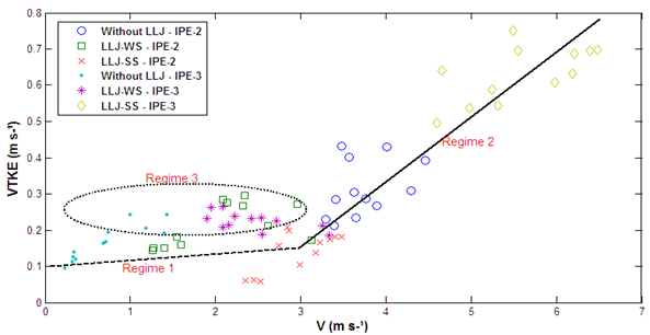Figure 5. Relation between turbulent intensity (VTKE) and wind velocity V for 6 distinct conditions regarding occurrence and season. The lines indicate three different turbulent regimes

Figure 5 presents a result based on methodology proposed by[4] and applied to Pantanal's data, for the six earlier mentioned cases. Each point in figure 5 represents a 5 minutes period inside 1 hour data intervals used above and presented in methodology section.

For the time interval of the -SS occurrence in flooded season it can be observed its values are well adjusted with regime 2. Such result confirms what was previously discussed (figure 2-f). That way, -SS action generates shear below the jet and intensifies turbulence already present in this period, which is due to the action of positive sensible heat flux, consequence of the water level presence (figure 4-f) in Pantanal surface. This was observed during the flooded season in Pantanal for -SS.

Another remarkable aspect of the result presented in figure 5 is the excellent agreement to what was presented by[4], according to the slope value associated to the regime 2 representative line. For Pantanal, a slope of approximately 0.24 was found, and reference[4] presents a slope of 0.25 to the representative line in regime 2.

It is also noted that the top-down mechanism action discussed above is well represented in regime 3, as expected from discussions in[4]. In cases where -WS and Without-, both in flooded season, top-down mechanism associated with GW caused these situations to appear, associated to regime 3. Top-down mixture action to -WS in dry season, as discussed in figure 4-c results , also generated occurrence of different events of this case in regime 3, supporting the discussed for this event. This way, an excellent agreement with turbulent regimes proposed by[4] and what was observed in this work to Pantanal NBL is remarked.

5. Conclusions

Three distinct conditions involving Low-Level Jets in Pantanal were studied (-ABSENT, -WS and -SS), to dry and flooded seasons. It has been observed that the occurrence of -SS in Pantanal's Nocturnal Boundary Layer may act as a blocking mechanism for the actions of great eddies with length scales higher than the jet's height. Such action is a clear manifestation of the shear-sheltering mechanism in Pantanal's NBL. On the other hand, -WS presence causes an intensification of top-down mechanisms actions. These actions are highlighted by the increase of contributions in the covariance between w and T and in their variances during periods subsequent to the detection of such type of .

Another interesting result comes from the unusual conditions prevailing in roughness of the Pantanal's experimental site with distinct surface roughness features, in dry and flooded seasons. Clear differences were observed in T variance's behavior for length scales lesser than 75m. During dry season, with greater roughness elements, clear spectral peaks in length scales smaller than 75m are noticed. During flooded season, with less roughness elements, these pikes are not present.

ACKNOWLEDGEMENTS

The authors wish to thank FAPESP (process Nº 98/00105-5) by financial support to the IPE project, to CNPq (process Nº 303.728/2010-8) by the research productivity grant provided to Leonardo Sá. The authors are also grateful to Federal University of Mato Grosso do Sul (UFMS) by the kindness to dispose a study base in the city of Corumbá in order to accomplish the IPE project; and to National Institute of Space Research (INPE) by its contribution in achieving IPE project, in its different stages. To Engineer Monica Pinheiro for their help with translation to English.