Edson R. Marciotto , Gilberto Fisch
Division of Atmospheric Sciences, Institute of Aeronautics and Space, São José dos Campos, 12228-904, Brazil
Correspondence to: Edson R. Marciotto , Division of Atmospheric Sciences, Institute of Aeronautics and Space, São José dos Campos, 12228-904, Brazil.
| Email: |  |
Copyright © 2012 Scientific & Academic Publishing. All Rights Reserved.
Abstract
The Alcântara Launch Center is located near the Brazilian Northeastern coastline downwind of a cliff 40 m high. Furthermore, the flow transition from open ocean past by the coastline generated an internal boundary layer (IBL) due to the roughness step change. The flow is mainly driven by the Trades, although the interaction with land-sea circulation may not be negligible. These features modify the ocean wind ocean profile as measured over land at the coastal site. We present here an ongoing research aiming to characterize the wind profile, which would serve as input flow profile in wind tunnel experiments and for gas dispersion studies. We analyzed the data of wind speed and direction collected between 1995 and 1999 by six aerovanes mounted in a 70-m height tower located about 200 m downwind the cliff. To study the diurnal and annual patterns of the wind profile the stored mean values of 10 min were monthly and hourly averaged. A simple estimate of the IBL height by assuming a dependence on the upwind distance of the shore as suggested in the literature were carried out. IBL height ranges from 30 to 40 m at tower location and being higher between 10 and 15 Local Time (LT). The wind profile power-law shows an alpha exponent greater (up to 0.35) than those encountered in the literature (about 0.10–0.11) for open ocean wind profile. The step change in the surface roughness cannot alone explain such a change in the alpha exponent. Other causes such as temperature step change and the cliff elevation certainly play a role to be still addressed.
Keywords:
Flow Past A Cliff, Ocean Wind Profile, Power Law Profile, Internal Boundary Layer Grow
Cite this paper: Edson R. Marciotto , Gilberto Fisch , Investigation of Approaching Ocean Flow and its Interaction with Land Internal Boundary Layer, American Journal of Environmental Engineering, Vol. 3 No. 1, 2013, pp. 18-23. doi: 10.5923/j.ajee.20130301.04.
1. Introduction
Sounding rockets for various scientific studies have been launched from the Alcântara Launch Center (ALC), and there are plans for launching the so-called VLS (Portuguese for Vehicle for Satellite Launching). The ALC is located at 2 19’ 03” N, 44 22’ 06” W, and about 200 m downwind from a coastal cliff, which is approximately 40 m high. Figure 1 shows two overviews of the ALC. The launch pad and the anemometric tower are at about the same distance from the cliff. The wind over the ALC is driven mainly by trade winds, but a land-sea circulation is also present. Besides the wind impact over the rockets trajectory, its structure, and safety during the launch, a general concern is about the dispersion of pollutant released from combustion of the propellants ([8],[10]). The determination of wind profiles is important in various studies in situ and also as input for numerical and physical models ([1],[13]).For example,[13] carried out direct numerical simulations (DNS) of a flow past a forward-facing step. Reference[1] performed a similar study but using a physical model in a wind tunnel. In both cases the idealized situation is that when the initial wind speed profile is similar to that found in the real case. Observations from the anemometric tower are used to obtain this incoming flow profile. However, the flow profile observed in this way is already perturbed. An ideal solution would be to take wind profile observations in an offshore area, say, 1 km from land-sea boundary. In the absence of the ideal solution, we tried to infer the incoming wind speed profile from the already perturbed wind profile collected by the anemometric tower through the analysis of its interaction with the internal boundary layer (IBL) developed inland. The vertical wind profile over the sea surface is an important quantity to take into account in many types of studies, such as estimates of heat and humidity flux, wind-driven waves, and loads on offshore structures. The logarithm wind profile has been extensively employed in the atmospheric surface boundary layer (SL) up to about 100 m above the sea level – asl ([4]). A reason to use a power-law instead of the logarithmic law is that, for practical applications, in situ measurements of the aerodynamic roughness length are not always possible, because it is related to both the wind speed and the wave characteristics of the ocean ([5]).Thus, the simplicity of the power-law wind profile is often preferred once it is quite accurate and useful for engineering purposes. The power-law can be written as | (1) |
Early studies by[3] and[5] determined α as equal to 0.10 for offshore sea surface. Later,[6] used a wider data range and recommended α = 0.11 ± 0.03. A review of the determination of α over ocean, including considerations of atmospheric stability is found in[7]. A relationship between α and z0 was proposed by[11] and it is given by | (2) |
z0 in meters. This gives us a value of z0 ≈ 1.1 10–3 m.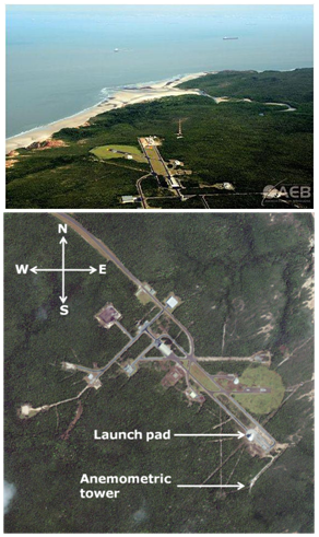 | Figure 1. (left) Overview the ALC, showing the launch pad, the anemometric tower, and the shore. The well defined line separating the vegetation area from the sand area evidence the presence of the 40-m high cliff. (right) Another overview of the ALC showing its position with respect to the cardinal points |
An equilibrium boundary layer develops only after the air has flowed over many individual obstacles or rows of obstacles. This roughness change problem has been well studied by[15] and correlations for the growth of the internal boundary layer are readily available; the internal boundary layer is the region of the flow that adjusts to the change of roughness. Within the internal boundary layer there is an equilibrium layer that can be broken into the new roughness sublayer and a new inertial sublayer.The study wind profile is fundamental for deriving parameters to be used in dispersion models. To study the wind regime at ALC we used five years of speed and direction wind data (from 1995-1999) collected at a six-level 70-m height tower. Diurnal and seasonal cycles were computed by averaging the data hourly and monthly.
2. Methodology
2.1. Roughness Step Change and IBL
When a flow passes by a roughness step change, an internal boundary layer starts to develop. Equilibrium boundary layer develops only after the air has flowed over sufficient fetch. In a laboratory study by[2] it was found that it takes about 300z0 for the equilibrium layer to reach the upper limits of the roughness sublayer. To apply the roughness-step-change approach on estimative of the internal boundary layer growth, we will disregard the coastal cliff, assuming the internal boundary layer is generated only by the roughness step change. Figure 2 sketches the flow over the cliff. 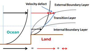 | Figure 2. Conceptual model of the development of the IBL. The transition layer between the internal and external layer is characterized by a greater slope and greater exponent α, such that αEBL < αIBL < αTL |
The equations for the wind speed profiles above and below the transition layer are: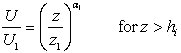 | (3) |
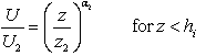 | (4) |
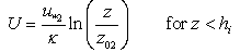
where hi is the IBL height, assumed to lie in the middle of the transition layer. Above the IBL the wind speed profile is likely to be the same as it was before passing over the coastal cliff. The reference heights z1 and z2 may be chosen as equal. In our particular case, we chose z1 = z2 = 70 m, which is the anemometric tower top-level. Similarly, we can write the logarithm-law profile as: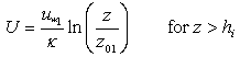 | (5) |
 | (6) |
It should be notice that due to the strong winds at ALC, the atmospheric stability is mostly near neutral. Reference [9] presented observations of the z / L which supports this assumption.The IBL height, hi, is given by | (7) |
with b = 0.38, from[12].
2.2. Inner and Outer Flow
One of the goals in this study is to try to recover the undisturbed ocean wind profile from the observation carried out at the coastal site (onshore). The idea behind is that if the IBL just formed were shallow enough, then the anemometers in highest levels would be being influenced only by the outer boundary layer, that is, the undisturbed ocean wind. Estimate αin and αout is possible in principle. The profile slope is related to α by mean of 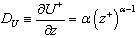 | (8) |
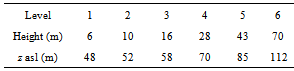
where U+ = U/Uref and z+ = z/zref. We can adopt the highest tower level as the reference height above the ground level, which is equivalent to 112 m above the sea level (Table 1). It is expected that the wind accelerates within the transition layer, because the outer flow is faster than the inner flow, making the wind speed profile to bend forward. Therefore, within the transition layer both the slope and exponent α must be greater than those found either in the internal boundary layer or in the external layer. Table 1. Levels and heights of aerovanes in the anemometric
 |
| |
|
3. Data
The wind data were collected from September 1995 to December 1999 by six aerovanes (Wind Monitor MA, Young, model 05106) installed in a tower 70-m high. The height above the ground level (agl) and above the sea level (asl) is given in Table 1. The tower and the aerovanes installed are shown in Figure 3. The primitive quantities collected are wind speed and wind direction stored each 10 minutes in a datalogger (CR7, Campbell Scientific). Hourly and monthly scalar averages were taken over the whole series in order to obtain mean diurnal and/or seasonal cycles.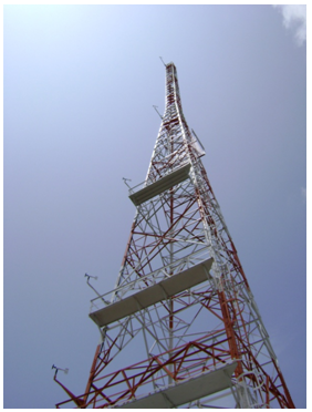 | Figure 3. View of the anemometric tower |
4. Results and Discussion
4.1. Wind Speed and Wind Direction
Figure 4(left) shows the wind speed as measured at level six (70 m agl). A remarkable seasonal variation especially during night and morning is observed, with amplitude of about 5 m/s. At early night the seasonal amplitude is only about 1.5 m/s. The diurnal cycle is less intense during the wet season, with a variation of 1 m/s, against 2 m/s during the dry season. The weakening of the diurnal cycle during the wet season is related to the decreasing of the thermal contrast between land and sea, which affects the land-sea breeze. However, it is not clear if this mechanism can explain a difference of up to 5 m/s as observed in the seasonal cycle. A displacement of the trade winds along the year could also be an important contribution. The diurnal cycle possess an opposite behavior for wet and dry season: wind speed during the wet season presents a maximum at early evening, whereas during the dry season a minimum is observed at early evening. A mean wind speed diurnal cycle would present a down concavity in the wet season and an up concavity in the dry season. In June and July, the transition season, the diurnal cycle is not well defined. Figure 4(left) suggests that a simple average over the diurnal cycle or over the seasonal cycle can be quite misleading. The result for the wind direction is shown in Figure 4 (right). The wind direction predominance is from E and NE. The wind trend to be rather from NE or even from NNE in the late afternoon in both seasons, and from ENE or from E in the morning during the transition season.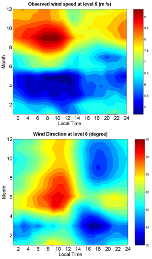 | Figure 4. (Above) Wind speed and (below) wind direction |
4.2. Power Law
Figure 5a shows mean diurnal and mean seasonal cycle of the exponent α fitted for a power-law profile using all six aerovanes in the tower. The diurnal cycle is better marked between January and June (the wet season), presenting lower values around 1200 LT. The values of α are not symmetrically distributed along the diurnal cycle since it is higher (less flat profiles) in the morning than in the afternoon. What can be inferred is that α departures from the lowest value at midday and increases systematically as time goes by until about 0800 LT of the next day, and then falls abruptly. This trend is kept for the dry season (July to December), but its amplitude is less. In the case of the seasonal cycle a maximum α is observed around July. At 1200 LT and around, an opposite behavior is observed, namely, α is minimal around July, especially in April and November. Note that the wind speed profile is flatter for lesser values of α. Wind profiles around midday are the flattest.It is not clear the origin of these flatter profiles; high resolution numerical modeling or physical modeling would be needed to better understand the flow over the coastal cliff and the resulting profile. As numerical modeling, we are in the phase of implementing a Large Eddy Simulation (LES), and in the field of physical modeling we have been employed wind tunnel simulations.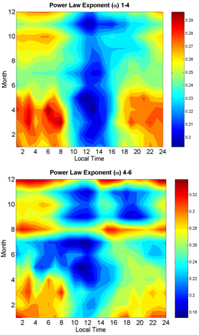 | Figure 5. Comparison of power-law exponent adjusted from the lowest levels (1-4) with that obtained from the highest levels (4-6) |
In order to study the disturbance of wind profile by the roughness step change, we estimated the IBL height (see next Section). Its values ranges from 28 m to 40 m, which correspond to tower level 4. Thus, to compute the exponent alpha we separate the whole profile in two: from levels 1 to 4 and from 4 to 6.The analysis of α obtained from adjustments using only levels 4 – 6 (Figure 5b) evidences that for most cases the IBL due to the roughness step change must be lower than 70 m. The basis for this conclusion is that α, and therefore, the slope, becomes greater when only the two or three top points are taken into account. In effect, the flow is being accelerated from the lower levels (1 – 4) to the upper levels (4 – 6), showing that the layer between levels 4 – 6 is still a flow transition layer of internal and external boundary layer. The prediction of IBL height by the formula proposed by[11] based just on a roughness step change (Eq. 2) may be not good enough to explain our observations; the cliff is likely to be altering the flow beyond the roughness step change effect.
4.3. Internal Boundary Layer
Besides the roughness step change, there are other two main factors affecting the IBL growing: (i) the topography, i.e., the change in the surface level and (ii) the surface temperature step change when the flow passes from the sea water to land. However, for simplicity and also for restriction in data we will address only the IBL growing due to a roughness step change, using the simple[12] parameterization.In order to investigate whether the observed wind is or is not an internal boundary layer flow, we estimate the internal boundary layer height based on the formula proposed by[12] (Eq. 7). However, instead of using the formula proposed by[11] (Eq. 2), which gives the roughness length straightforward as function of α, we obtained z0 from the log-law fit, setting the displacement of zero-plane height, d0, equals zero. Figure 6 shows the IBL height estimated in this way, using a fetch of 200 m. The IBL height seems to be well anti-correlated with the exponent α as suggested by Eqs. 2 and 7 and varies in the range of 28 – 40 m. Accordingly, the aerovane at the highest level would never be influenced by the wind developed in the IBL generated only by the roughness step change. 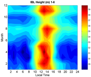 | Figure 6. The IBL height computed from Eq. 7 using the all six tower level |
A well defined anti-correlation was found between IBL height and α obtained with all levels or only levels 1 – 4, but not with levels 4 – 6 only (compare Figs 5a and 6). A shear transition layer is formed between the internal and external boundary layer. In this layer the flow must be speeding-up, which results the increase of the slope du/dz, and consequently the increase of the exponent. Below the transition layer α is smaller.Figure 7 shows a vertical profile of a particular case: August at 0900 LT of Figure 6. zinf is the tower level of 70 m and Uinf is the speed at this level. We see that the slope changes according to the levels taken into account to compute α. For this case we can infer the presence of a three-layer flow, like in our conceptual model.
5. Summary and Future Work
Wind speed and direction collected at a six-level tower from 1995 to 1999 were used to study their variation and to assess their properties. The site is the Alcântara Launch Center in the coastal area in the northeast Brazil, and is located nearby the equatorial line (2 degrees South), being under the influence of the trade winds. The wind speed profile can be described adequately by means of a power-law. The exponent α ranges from 0.19 to 0.29 for the four first levels and from 0.18 to 0.33 for the three highest levels. Greater values of α in highest levels indicate that the flow is accelerating in a layer which is probably a transition layer between internal and external boundary layer. This transition layer is characterized by a higher wind-shear. In addition, the exponent α obtained from upper levels does not follow exactly the alpha pattern for lower levels, which is systematically higher, suggesting a decoupling of the flow. A simple estimation of the IBL height assuming a roughness step change provides a value ranging from about 50 to 70 m. The visual inspection of some individual wind profile shows that a three-layer flow occurs in some occasions and that they are consistent with the our conceptual model of a flow past a roughness step change.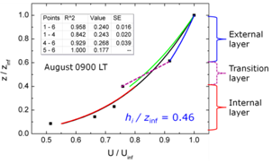 | Figure 7. Vertical profile for August at 0900 local time. A three-layer flow can be noticed |
As future work further measurements must be carried out to address open question in this preliminary study: how the topography affects the wind profile? What is the effect of the thermal step change on the IBL growing? Inland measurement up to 200 m using an existing mini-sodar is ongoing and can be very useful to understand the modification of the ocean flow as it approaches land. Knowing the shape of the undisturbed flow will be important to set-up wind tunnel simulations of structure loads and pollutant dispersion.
ACKNOWLEDGEMENTS
The authors thank Fundação de Amparo à Pesquisa do Estado de São Paulo (FAPESP), Grant 2010/16510-0, and Conselho Nacional de Desenvolvimento Científico e Tecnológico (CNPq), Grant Universal 471143/2011-1.
References
| [1] | A.C. Avelar, J.R. Banhara, N.R. Fico Jr., C.R. Andrade, E.L. Zaparoli, “Experimental and numerical investigation of roughness and three-dimensional effects on the flow over shallow cavities”, 39th AIAA Fluid Dynamics Conference 22 - 25 June 2009, San Antonio, Texas. |
| [2] | H. Cheng, I.P. Castro, “Near-wall flow development after a step change in surface roughness”, Bound-Layer Meteorol., 6, 1-21, 2001. |
| [3] | A.G. Davenport, “The relationship of wind structure to wind loading”, National Physical Laboratory, Symposium number 16, Wind effects on building and structures, 54-102, 1965. |
| [4] | J.R. Garratt, “The Atmospheric Boundary Layer”, Cambridge University Press, 1994. |
| [5] | S.A. Hsu, “Coastal Meteorology”, Academic Press, 1988. |
| [6] | S.A. Hsu, E.A. Meindl, D.B. Gilhousen, “Determining the power-law wind-profile exponent under near-neutral stability condition at sea”, J. Appl. Meteorol. Climatol., 33, 757-765, 1994. |
| [7] | S.A. Hsu, B.W. Blanchard, “Recent advances in air–sea interaction studies applied to overwater air quality modeling: a review”, Pure Appl. Geophys., 160, 297-316, 2003. |
| [8] | E.R. Marciotto, G. Fisch, L.E. Medeiros, “Characterization of surface level wind in the Centro de Lançamento de Alcântara for use in rocket structure loading and dispersion studies”, J. Aerospace Tech. Manag., 4, 69-79, 2012. |
| [9] | R. Magnago, G. Fisch, O. Moraes, “Análise espectral do vento no Centro de Lançamento de Alcântara (CLA)”, Rev. Bras. Meteorol., v.25, 260-269, 2010. |
| [10] | D.M. Moreira, L.B. Trindade, G. Fisch, M.R. Moraes, R.M. Dorado, R.L. Guedes, “A multilayer model to simulate rocket exhaust clouds”, J. Aerospace Tech. Manag., 3, 41-52, 2011. |
| [11] | H.A. Panofsky, J.A. Dutton, “Atmospheric Turbulence”, Wiley, 1984. |
| [12] | W. Pendergrass, S.P.S. Arya, “Dispersion in neutral boundary layer over a step change in surface roughness – I. Mean flow and turbulence structure”, Atmos. Environ., 18, 1267-1279, 1984. |
| [13] | L.B. Pires, “Estudo da camada limite interna desenvolvida em falésias com aplicação para o Centro de Lançamento de Alcântara”, Ph.D Thesis, Instituto de Pesquisas Espaciais (INPE), São José dos Campos, 2009. |
| [14] | S.C. Pryor, R.J. Barthelmiea, “Statistical analysis of flow characteristics in the coastal zone”, J. Wind Eng. Ind. Aerodyn., 90, 201-221, 2002. |
| [15] | A.J. Smits, D.H. Wood, “The response of turbulent boundary layers to sudden perturbation”. Annu. Rev. Fluid Mech. 17, 321-358, 1985. |
 Abstract
 Reference
 Full-Text PDF
 Full-text HTML