Bianca Luhm Crivellaro 1, Nelson Luís Dias 2, Tomás Chor 1
1Graduate Program in Environmental Engineering (PPGEA), Federal University of Parana (UFPR), Curitiba, 81531-990, Brazil
2Department of Environmental Engineering, Federal University of Parana (UFPR), Curitiba, 81531-990, Brazil
Correspondence to: Nelson Luís Dias , Department of Environmental Engineering, Federal University of Parana (UFPR), Curitiba, 81531-990, Brazil.
| Email: |  |
Copyright © 2012 Scientific & Academic Publishing. All Rights Reserved.
Abstract
A field experiment designed to test sensor separation effects by means of multiple thermocouple measurements co-located with a sonic anemometer, a fast gas analyzer and a slow set of CO2 and humidity sensors is described. The data allowed the experimental determination of decorrelation between scalars, both because of instrumental effects (mostly sensor separation) and physical ones (mostly large-scale ABL processes associated with flux entrainment at the top). The large-scale effects are more important in terms of the decorrelation they produce, and yet their effect on the measured fluxes is not too large, on account of the high-pass filtering nature of the multiplication by the vertical velocity fluctuation, with its inherently higher-frequency range.
Keywords:
Scalar Similarity, Sensor Separation, Turbulent Fluxes
Cite this paper: Bianca Luhm Crivellaro , Nelson Luís Dias , Tomás Chor , Spectral Effects on Scalar Correlations and Fluxes, American Journal of Environmental Engineering, Vol. 3 No. 1, 2013, pp. 13-17. doi: 10.5923/j.ajee.20130301.03.
1. Introduction
It is important to establish how similar scalars are in the turbulent atmospheric surface layer for several reasons. Many models and measurement techniques rely on the assumption that scalars are perfectly similar, for example SVATs ([1],[2]), the widely applied Energy-Budget Bowen Ratio Method (e.g.[3],[4]) and the bandpass eddy covariance method ([5]).In spite of its widespread use, however, it has long been known that in practice perfect similarity does not hold ([6-9]). Most of these evaluations report values of the bulk correlation coefficient between two scalars, | (1) |
where  is Reynolds’ decomposition, and
  is the standard deviation of a.However, very seldom a detailed description is made of the scalar correlation being reported (exceptions, for example, are[5] and more important[10]).There are several causes that act to decorrelate scalars. They are both instrumental (sensor accuracy, response time and spatial separation) and physical, such as local advection, surface patchiness and large-scale atmospheric boundary layer (ABL) effects.In this work, we report a short experiment where a very detailed sensor setup was put in place to resolve small-scale decorrelation effects due to sensor separation, and where large-scale effects could be identified by standard Fourier methods.Band-pass spectral analyses allow the identification of the frequency ranges affected, respectively, by large-scale boundary-layer effects, surface layer scaling that follows the Monin-Obukhov Similarity Theory (MOST), and small-scale effects.The analyses show that(a) Large-scale ABL processes are the most important for scalar variance and fluxes; each scalar is affected differently, likely because their entrainment fluxes at the top of the ABL are different.(b) Because of the high-pass filtering nature of the product with the vertical velocity fluctuations that is inherent in the calculation of the scalar fluxes, however, the fluxes themselves are much less influenced by (a), as can be inferred from the higher relative transfer efficiencies in comparison with the correlation coefficients.(c) Sensor separation is less important, and affects fluxes slightly less than it affects scalar covariances.
2. Experimental Apparatus
The data were measured at a grass farm in Tijucas do Sul, PR, Brazil, latitude 25°50’07.12” S, longitude 49°07’47.77” W and altitude 900 m, from February 16 thru February 27, 2011. A CSI (Campbell Scientific Instruments) CSAT-3 three-dimensional sonic anemometer was deployed at 1.85 m above the grass in a favorable fetch direction: during the experiment, the wind blew from NE 85% of the time.It was a very rainy period, and data loss due to rain was high: only 20% of the measured runs were “dry” (as revealed by careful data screening and inspection of the CSAT-3 quality-control flags). Only those runs are reported here, and only for daytime unstable conditions when the fetch was adequate.On both sides of the CSAT-3 were deployed a “fast” and a “slow” set of sensors. The “fast” set consisted of a Licor LI-7500 open-path gas analyzer measuring H2O, CO2 and pressure. A fine-wire thermocouple (Campbell FWTC3) was mounted with the measuring head located in the middle of the LI-7500 measuring path. The “slow” set consisted of Vaisälä GMP343 CO2 sensor, a Campbell Sci CS500 H2O and temperature sensor, and 2 FWTC3 thermocouples, mounted with their heads as close as possible to each sensor. Results from the “slow” set of sensors are not reported here.All data were logged on a Campbell Sci CR23-X datalogger at 20 Hz and stored on a netbook running continuously on battery power, with an in-house Python program reading the binary data (in CSI format) directly from the CR23-X RS-232 port.The raw turbulence data were stored in a new file every 10 minutes, but here all analyses are performed on 1-hour runs obtained by merging every six 10-min. data available, so as to maximize the number of runs for analysis. Each run is labeled by the ending time of the last 10-min. period within it.
3. Methods
We denote the cross-spectrum between two turbulent fluctuations a and b by | (2) |
where n is cyclic frequency,  is the cospectrum,
  is the quadrature spectrum, and
  . In the following, all lowercase quantities indicate the turbulent fluctuation.
  means the temperature measured by the thermocouple co-located with the CSAT3;
  the temperature measured by the thermocouple co-located with the LI7500; q the specific humidity measured by the LI7500; c the CO2 mass concentration measured by the LI7500; w the vertical velocity, and u the longitudinal velocity. The spectral correlation coefficient is then given by
 | (3) |
Each spectrum/cross-spectrum is calculated as a composite of six 10-min. blocks and thirty 2-min. blocks (see[11]), in a compromise to estimate the low-frequency components down to 10min-1 reasonably well, and at the same time to obtain low-variability in the spectral densities in the higher frequencies.Block averaging over 1 hour and subtraction from the hourly average was used to extract the fluctuations which were then submitted to spectral analysis: no high-pass filtering was applied, in order not to distort the low-frequency range behavior of the cross-spectra. Notice however that, as the end result are composite spectra representative of a 1-hour period, but whose lowest frequency is 10min-1, the statistics calculated from numerical integration of these spectra are somewhat similar to block averaging successive 10-min. blocks within the hour, and extracting fluctuations around each of the 10-min averages.Our approach, motivated by the work of[5], is to calculate variances/covariances over frequency bands in the spectral domain, each of which is of the form | (4) |
All scalar covariances and fluxes in this work, including the friction velocity needed to obtain Obukhov’s stability variable ζ, are calculated in this way. No corrections for density effects (the so-called WPL correction ([12]) were applied to the calculated fluxes, not because they are not important numerically, but because we wanted to concentrate our attention on the classic turbulent part of the flux, of the form
  , and to the scalar variances/covariances, of the form
  . Any corrections to these quantities taking into account the effects studied in the present work will then carry over to flux estimates further corrected, if desired, to density effects by means of the WPL equations.
4. Results
Figure 1 shows the spectral correlation coefficient  for the 1-hr run ending at Feb 17, 2011 at 15:20 h. Note the distinctive fall-off starting at n = 0.1Hz. This is with all probability due to the ~ 0.2m transversal separation between the CSAT-3 and the LI-7500.
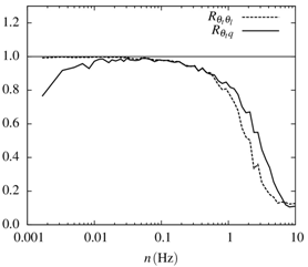 | Figure 1. Spectral correlation coefficients and and showing the effects of sensor separation showing the effects of sensor separation |
If two scalars, say, temperature and humidity, are measured in the surface layer, such separation is unavoidable on account of the finite size of each sensor. Thus, in the same figure we see the very similar behavior of . Notice however that the LI7500 averages over its path, so the two lines in Figure 1 are not completely comparable.The simultaneous thermocouple measurements allow the calculation of the loss of correlation due to sensor separation, as well as the corresponding sensible heat flux loss. Also, since the low-frequency range is unaffected by this effect, remaining as it should very close to 1 in the case of
  , these temperature measurements provide the best way to assess the consequences of sensor separation experimentally. The measured bulk correlation coefficient will be affected by this separation, and the naive estimate, that doesn’t account for it, will be
 | (5) |
where Ny = 10Hz is the Nyquist frequency. If we assume that there are no other flux losses other than those produced by sensor separation, the flux loss can be calculated (in the case of the sensible heat flux, and for our experimental setup) by | (6) |
In Figure 2, we plot both  and
and  as a function of Obukhov’s stability variable ζ. As expected for unstable conditions, where no systematic behavior of the scalar spectra characteristic frequencies with ζ has been observed[13], there is no systematic dependence of either variable with stability.
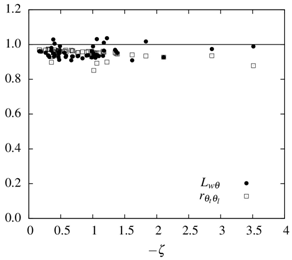 | Figure 2. Sensor separation effects on scalar bulk correlation and scalar flux |
The observed loss is small, amounting to no more than 5% on the average, but it may be significant in some situations.The low-frequency range of the scalar spectra and cospectra has a much more important decorrelation behavior. This is a real phenomenon, not an experimental setup artifact, and can only be observed with different scalars. Although no direct verification of the cause for this decorrelation can be obtained with the present dataset, the most likely cause are the large-scale ABL processes related to the scalars’ entrainment fluxes at its top. This reasoning can be given further support, in our case, by the fact that the surface over which the measurements were taken is very homogeneous; therefore, surface flux variability such as identified by[7] and[14] is unlikely to play a role here.The effect is clearly seen in Figure 3, with different fall-offs for  and
and  , while both start at essentially the same cutoff frequency, n ~ 0.01Hz.In contradistinction, all our runs show an intermediate range, 0.01–0.1 Hz, where
 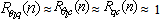 . This is the expected behavior from MOST ([6],[15]).
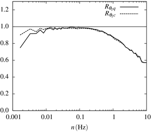 | Figure 3. Low- and high-frequency fall-off of the spectral correlation coefficient between pairs of different scalars |
We now use the results from the spatially separated thermocouples and use, as our best (“corrected”) estimates for  :
: | (7) |
where Nc = 0.1Hz is the cutoff frequency (visually identified) where separation effects and the corresponding fall-off from 1.0 starts to appear in the scalar spectral correlation functions. In Figure 4, we plot  . Note that the correction increases the correlation coefficients significantly, close to 1. Again, no systematic trend with stability can be discerned.In order to investigate whether the smaller values of
  observed in Figure 4 might be related to the daytime evolution of the atmospheric boundary layer, the correction procedure outlined and tested above for the correlation between temperatures (where the outcome of +1 is known exactly) was extended to the correlation coefficients
  and
and  . The results are shown in Figure 5 as a function of the time-of-day, between sunrise and sunset, during the experiment.
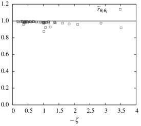 | Figure 4. Corrected scalar correlation as a function of stability, showing the effect of the low-frequency decorrelation caused (possibly) by large-scale processes |
The use of time-of-day for the x-axis was based on the assumption that, as the ABL evolves through the day, this could have an impact on the low-frequency range of  and
and  which is responsible for less-than-perfect correlation. However, this is not confirmed in Figure 5. Instead, the correlations seem to remain constant throughout the day for both temperature-water vapor and temperature-CO2. Clearly, there is more variability in the former, which also tends to be lower. This may be connected to the fact that during daytime the entrainment fluxes of sensible heat and CO2 at the top of the ABL have the same time, thus improving scalar similarity throughout the ABL, whereas the entrainment fluxes of sensible heat and water vapor have opposing signs, with the opposite effect.
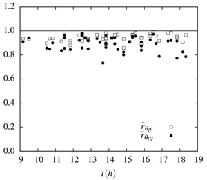 | Figure 5. Daytime march of the scalar correlation coefficient |
5. Conclusions
In this work we applied a systematic procedure to identify scale effects on scalar-scalar, and vertical velocity-scalar, correlations. Small-scale, separation effects, are important as seen in the usual log-scale plots of spectral correlation coefficients. It should of course be taken into account whenever possible, but the fact is that they are not very important on the bulk covariances (both scalar-scalar and vertical velocity-scalar).The low frequencies, on the other hand, display scalar-specific behavior that can be traced to the entrainment fluxes at the top of the ABL. They reduce scalar correlation coefficients appreciably, but have a smaller direct effect on the calculated scalar fluxes, given the fact that the product with w already “high-pass” filters the wa covariances.
References
| [1] | J. C. Calvet, J. Noilhan, J. L. Roujean, P. Bessemoulin, M. Cabelguenne, A. Olioso and J. P. Wigneron. An interactive vegetation SVAT model tested against data from six contrasting sites. Agricultural and Forest Meteorology, 92:73–95, 1998. |
| [2] | R. Avissar and R. A. Pielke. A parameterization of heterogeneous land surface for atmospheric numerical models and its impact on regional meteorology. Montly Weather Review, 1989. |
| [3] | R. J. Reis and N. L. Dias. Multi-season lake evaporation: energy-budget estimates and crle model assessment. Journal of Hydrology, 208:135–147, 1998. |
| [4] | N. G. Lensky, Y. Dvorkin, V. Lyakhovsky, I. Gertman and I. Gavrieli. Water, salt and energy balances of the dead sea. Water Resource Researh, 41:W12418, 2005. |
| [5] | J. Asanuma, H. Ishikawa, I. Tamagawa, Y. Ma, T. Hayashi, Y. Qi and J. Wang. Application of the band-pass covariance technique to portable flux measurements over the Tibetan Plateau. Water Resource Research, 41(W09407), 2005. |
| [6] | R. J. Hill. Implications of Monin-Obukhov similarity theory for scalar quantities. Journal of the Atmospheric Sciences, 46:2236–2244, 1989. |
| [7] | H. A. R. de Bruin, W. Kohsiek and J. J. M. van der Hurk. A verification of some methods to determine the fluxes of momentum, sensible heat and water vapor using standard deviation and structure parameter of scalar meteorological quantities. Boundary-Layer Meteorology, 63:231–257, 1993. |
| [8] | J. Asanuma and W. Brutsaert. Turbulence variance characteristics of temperature and humidity in the unstable atmospheric surface layer above a variable pine forest. Water Resource Research, 35(2):515–521, 1999. |
| [9] | G. G. Katul and Cheng-I Hsieh. A note on the flux-variance similarity relationships for heat and water vapour in the unstable atmospheric surface layer. Boundary-Layer Meteorology, 90:327–338, 1999. |
| [10] | J. Asanuma, I. Tamagawa, H. Ishikawa, Y. Ma, T. Hayashi, Y. Qi and J. Wang. Spectral similarity between scalars at very low frequencies in the unstable atmospheric surface layer over the tibetan plateau. Boundary-Layer Meteorology, 122:85–103, 2007. |
| [11] | J. S. Bendat and A. G. Piersol. Random Data. John Wiley & Sons, New York, 2 edition, 1986. 566 pp. |
| [12] | E. K.Webb, G. I. Pearman and R. Leuning. Correction of flux measurements for density effects due to heat and water vapor transfer. Quarterly Journal of the Roy Meteorology Society, 106:85–100, 1980. |
| [13] | J. C. Kaimal, J. C. Wyngaard, Y. Izumi and O. R. Coté. Spectral characteristics of surface-layer turbulence. Quarterly Journal of the Roy Meteorology Society, 98:563–589, 1972. |
| [14] | J. Asanuma and W. Brutsaert. The effect of chessboard variability of the surface fluxes on the aggregated turbulence fields in a convective atmospheric surface layer. Boundary-Layer Meteorology, 91:37–50, 1999. |
| [15] | N. L. Dias and W. Brutsaert. Similarity of scalars under stable conditions. Boundary-Layer Meteorology, 80:355–373, 1996. |
 Abstract
 Reference
 Full-Text PDF
 Full-text HTML