Jonas C. Carvalho 1, Marco T. M. B. Vilhena 2, Gervásio A. Degrazia 3, Marieli Sallet 1
1Universidade Federal de Pelotas, Pós-Graduação em Meteorologia, Pelotas, RS, Brazil
2Universidade Federal do Rio Grande do Sul, Pós-Graduação em Eng. Mecânica, Porto Alegre, RS, Brazil
3Universidade Federal de Santa Maria, Pós-Graduação em Meteorologia, Santa Maria, RS, Brazil
Correspondence to: Jonas C. Carvalho , Universidade Federal de Pelotas, Pós-Graduação em Meteorologia, Pelotas, RS, Brazil.
| Email: |  |
Copyright © 2012 Scientific & Academic Publishing. All Rights Reserved.
Abstract
In this work we present a semi-analytical Lagrangian particle model to simulate the pollutant dispersion during low wind speed conditions. The model is based on a methodology, which solves the Langevin equation through the assumption that coefficient of the integrating factor is a complex function. The method leads to a non-linear stochastic integral equation, which is solved by the Method of Successive Approximations or Picard’s Iterative Method. Taking into account the isomorphism between the complex and real plane by writing down the low wind formulation in polar form, the procedure allow to determine a formula for the low wind direction. Furthermore, an expression analogous to the Eulerian autocorrelation function suggested by Frenkiel[1] appears in the real component solution. The model results present an improvement in relation to the other models and are shown to agree very well with the field tracer data collected during stable conditions at Idaho National Engineering Laboratory (INEL).
Keywords:
Low Wind Speed Condition, Air Pollution Modelling, Lagrangian Particle Model, Picard Iterative Method, Autocorrelation Function, Model Evaluation
Cite this paper: Jonas C. Carvalho , Marco T. M. B. Vilhena , Gervásio A. Degrazia , Marieli Sallet , A General Lagrangian Approach to Simulate Pollutant Dispersion in Atmosphere for Low-wind Condition, American Journal of Environmental Engineering, Vol. 3 No. 1, 2013, pp. 8-12. doi: 10.5923/j.ajee.20130301.02.
1. Introduction
Recent years have been seen the flowering of the work of searching analytical solution for the Langevin equation with the main purpose of simulating pollutant dispersion in the atmosphere. The meaning of analyticity relies on the fact that no approximation is made in the derivatives or domain discretization along the solution derivation. In this direction, appeared in the literature the works of Carvalho et al.[2-3], which solves the Langevin equation by the following steps: linearization of the Langevin equation and solution of the resultant stochastic integral equation by the Picard iterative scheme. This procedure leads to an analytical solution in each iterative step. Carvalho and Vilhena[4] solved by this methodology the Langevin equation for low wind speed condition. In order to model the pollutant dispersion during meandering effect in the solution, the authors made the assumption that the coefficient of the integrating factor of the first order linear differential equation is a complex function, the imaginary component models the low wind condition. Furthermore, the authors considered only the real component of the integrating factor. At this point, it is relevant to mention that by this procedure, the Frenkiel[1] autocorrelation function naturally appears in the solution.In this work we obtain a more general model, unlike the work of Carvalho and Vilhena[4], considering the real and imaginary parts of the complex function before performing the multiplication of the integrating factor, expressed by the Euler formula, inside and outside of the integral solution. Taking into account the isomorphism between the complex and real plane by writing down the low wind formulation in polar form, the procedure allow to determine a formula for the low wind direction. Furthermore, an expression analogous to the Eulerian autocorrelation function suggested by Frenkiel[1] appears in the real component solution. Finally, it is necessary to mention that when the non-dimensional quantity that controls the meandering oscillation frequency goes to zero this solution reduces to the solutions encountered by Carvalho et al.[2-3] for windy condition. The low wind speed data collected during stable conditions at Idaho National Engineering Laboratory (INEL)[5] has been used to evaluate the new model. The paper is outlined as follows: in section two the model is presented, in section three the modelling results are discussed and in section four the conclusions.
2. The Low Wind Model
The approach consists in the linearization of the Langevin equation as stochastic differential equation: | (1) |
which has the well known solution in terms of the integrating factor: | (2) |
In order to embody the low wind speed condition in the Langevin equation, it is assumed that  and
and  are complex functions written as:
 | (3) |
and | (4) |
where  and
and  are the real and imaginary parts of
  , respectively, and
  and
and  are the real and imaginary parts of
  , respectively. Therefore, the exponentials appearing in Equation (2) reads like:
 | (5) |
Applying the Euler formula, Equation (2) becomes: | (6) |
Multiplying the Equation (6) by the complex conjugate and performing the multiplications, we can obtain | (7) |
Considering  , we can write the Equation (7) as
 | (8) |
In order to determine the wind direction we cast equation (8) into: | (9) |
where by comparison with Equation (3) we have | (10a) |
and | (10b) |
Bearing in mind the isomorphism between the complex and real planes, the low wind expression given by Equation (9) is described in the complex plane. This procedure allows as determining the low wind direction, using polar form. For this end, we rewrite Equation (9) like | (11) |
where  is the low wind direction relative the x-axis
 | (12) |
Note that the real component of the Equation (9),  is analogous to the Eulerian autocorrelation function suggested by Frenkiel[1] (p. 80) and written in a different way by Murgatroyd[6]. Therefore,
  and
and  are given by
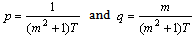 where
where  is the time scale for a fully developed turbulence and
  is a non-dimensional quantity that controls the meandering oscillation frequency. At this point, it is important to mention that when
  goes to zero the Equation (9) reduces to the solution for windy conditions, which is written in terms of the exponential form of the autocorrelation function.The Equation (9) is a non-linear stochastic integral equation, which must be solved iteratively. The method applied to solve the Equation (9) is the Method of Successive Approximations or Picard’s Iteration Method[7], assuming that the initial guess for the iterative approximation is determined from a Gaussian distribution. For applications, the values for the parameters
  and
and  have been calculated according to Carvalho et al.[8]:
 | (13) |
and | (14) |
where  is the stable PBL height,
  is the friction velocity and
  .As the turbulence is considered Gaussian in the horizontal direction, the function
  can be given by:
 | (15) |
where  is the turbulent velocity variance,
  is the Lagrangian time scale and
  is a normally distributed (average 0 and variance
  ) random increment. For the vertical component, we solve the Langevin equation by the ILS approach as suggested by Carvalho et al.[4].
3. Modelling Results
The data utilized to evaluate the model performance are composed by a series of field experiments conducted under stable conditions in low winds over flat terrain. The tracer data were collected at Idaho National Engineering Laboratory (INEL) and the results are published in a U.S. National Oceanic and Atmospheric Administration (NOAA) report[5].For the simulations, the turbulent flow is assumed inhomogeneous only in the vertical and the transport is realized by the longitudinal component of the mean wind velocity. The horizontal domain was determined according to sampler distances and the vertical domain was set equal to the observed PBL height. The time step was maintained constant and it was obtained according to the value of the Lagrangian decorrelation time scale ( ), where
  must be the smaller value between
  (with
(with  ) and
) and  is an empirical coefficient set equal to 10. The values of
  and
and  were parameterized according to scheme developed by Degrazia et al.[9]. The integration method used to solve the integrals appearing in Equation (10) was the Romberg technique. Because of wind direction variability during the INEL experiment, a full 360o sampling grid was implemented. Arcs were laid out at radii of 100, 200 and 400 m from the emission point. Samplers were placed at intervals of 6o on each arc for a total of 180 sampling positions. The receptor height was 0.76 m. The tracer SF6 was released at a height of 1.5 m. The 1 h average concentrations were determined by means of an electron capture gas chromatography. Wind measurements were provided by lightweight cup anemometers and bivanes at the 2, 4, 8, 16, 32 and 61 m levels of the 61-m tower located on the 200 m arc. Table 1 shows the meteorological data utilized for the validation of the proposed model. Observed wind speeds were used to calculate the coefficients for the exponential wind profiles. The Monin-Obukhov length
  and the friction velocity
  were approximated through the numerical best fit between the observed wind speeds and calculated wind profile suggested by Businger et al.[10]. To calculate h (the stable PBL height), the relation
  was used[11], where
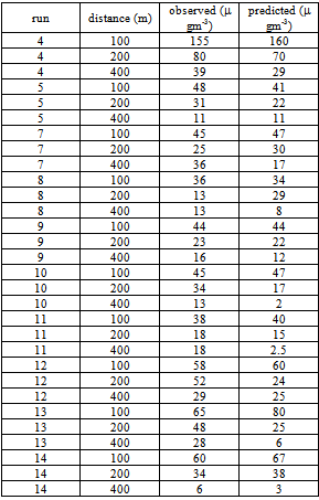
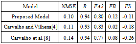
  is the Coriolis parameter.The model performance is shown in Tables 1 and 2 and Figures 1. Table 1 shows the comparison between observed and predicted ground-level centerline concentrations. Table 2 presents the result of the statistical analysis made with observed and predicted values of ground-level centerline concentration following Hanna’s[12] statistical indices. Giving a look at the results we observe that the model simulates quite well the experimental data in stable condition and, indeed, presents results comparable or even better than ones obtained by Carvalho and Vilhena[4] and Carvalho et al.[8]. The statistical analysis reveals that all indices are within acceptable ranges, with NMSE, FB and FS values are relatively near to zero and R and FA2 are relatively near to 1.
 Table 1. Observed and predicted ground-level centerline concentrations
 |
| |
|
Table 2. Statistical evaluation
 |
| |
|
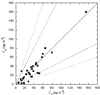 | Figure 1. Scatter diagram between observed (Co) and predicted (Cp) ground-level centerline concentration. Dashed lines indicate factor of 2, dotted lines indicated factor of 3 and solid line indicates unbiased prediction |
4. Conclusions
In this paper was presented a more general model to simulate the pollutant dispersion in meandering low wind conditions. The model was obtained by solving the Langevin equation through the integrating factor with its coefficient being a complex function. The method leads to a stochastic integral equation whose solution was obtained through the Method of Successive Approximations or Picard’s Iteration Method. Taking into account the isomorphism between the complex and real plane by writing down the low wind formulation in polar form, it was possible to determine a formula for the low wind direction. An expression analogous to the Eulerian autocorrelation function for meandering conditions appeared in the real component solution. The proposed method can be used to simulate de contaminant dispersion in meandering or non-meandering situations. The model was evaluated through the comparison with experimental data. The results obtained by the new model agree very well with the experimental data, indicating that it represents the dispersion process correctly in low wind speed conditions.
ACKNOWLEDGEMENTS
The authors acknowledge the financial support provided by CNPq. (Conselho Nacional de Desenvolvimento Científico e Tecnológico) and CAPES (Coordenação de Aperfeiçoamento de Pessoal de Nível Superior).
References
| [1] | François N. Frenkiel, "Turbulent diffusion: Mean concentration distribution in a flow field of homogeneous turbulence", Advances in Applied Mechanics, vol.3, pp.61-107, 1953. |
| [2] | Jonas C. Carvalho, Ézio R. Nichimura, Marco T. M. B. Vilhena, Davidson M. Moreira, Gervásio A. Degrazia, "An iterative langevin solution for contaminant dispersion simulation using the Gram-Charlier PDF", Environmental Modelling and Software, vol.20, no 3, pp. 285-289, 2005. |
| [3] | Jonas C. Carvalho, Marco T. M. B. Vilhena and Davidson M. Moreira, "An alternative numerical approach to solve the Langevin equation applied to air pollution dispersion", Water, Air and Soil Pollution, vol.163, no 1-4, pp. 103-118, 2005. |
| [4] | Jonas C. Carvalho, Marco T. M. B. Vilhena, "Pollutant dispersion simulation for low wind speed condition by the ILS method", Atmospheric Environment, vol.39, pp.6282-6288, 2005. |
| [5] | Jerrold F. Sagendorf, C. Ray Dickson, "Diffusion under low wind-speed, inversion conditions", U.S. National Oceanic and Atmospheric Administration Tech. Memorandum ERL ARL-52, 1974. |
| [6] | R. J. Murgatroyd, Estimations from geostrophic trajectories of horizontal diffusivity in the mid-latitude troposphere and lower stratosphere, Quarterly Journal of the Royal Meteorological Society, vol.95, pp.40-62, 1969. |
| [7] | W. Boyce, R. DiPrima, 2001. Elementary differential equations and boundary value problems, Wiley, New York, 749 pp, 2001. |
| [8] | Jonas C. Carvalho, Gervásio A. Degrazia, Sérgio G. Magalhães, "Parameterization of meandering phenomenon in a stable atmospheric boundary layer", Physica A, vol.368, pp.247-256, 2006. |
| [9] | Gervásio A. Degrazia, Osvaldo L. L. Moraes, Amauri P. Oliveira, "An Analytical method to evaluate mixing length scales for the planetary boundary layer", Journal of Applied Meteorology, vol.35, pp.974-977, 1996. |
| [10] | J. A. Businger, Turbulent transfer in the atmospheric surface layer. In D.A. Haugen (Ed.), Workshop in Micrometeorology, American Meteorological Society, Boston, pp.67-100, 1973 |
| [11] | Sergei S. Zilitinkevith, On the determination of the height of the Ekman boundary layer. Boundary-Layer Meteorology vol.3, pp.141-145, 1972. |
| [12] | Steven R. Hanna, "Confidence limit for air quality models as estimated by bootstrap and jacknife resampling methods", Atmospheric Environment, vol.23, pp.1385-1395, 1989. |
 Abstract
 Reference
 Full-Text PDF
 Full-text HTML