1. Introduction

This study aimed to evaluate the performance of four turbulence parameterization schemes available in the Brazilian Developments on the Regional Atmospheric Modeling System - BRAMS[1-2] - model for a simulated case of a Squall Line occurred on the Metropolitan Area of São Paulo (MASP) and choose the parameterization of turbulence that possibly best represents this kind of phenomena.

One characteristic of urban areas such as MASP is the large number of problems faced during the spring and summer seasons due to the occurrence of severe weather, like thunderstorms, common in most days in the late afternoon and early evening. Some of these storms are responsible for floods, landslides, falling trees and metal structures, unroofing of houses and often can cause human losses[3,4]. The formation of these storms may be associated with various meteorological phenomena, such as: Mesoscale Convective Systems (MCS), in particular, the Squall Lines[3].

In recent years some papers were published on the performance of turbulence parameterization schemes such as[6] that analyzed the impact of three different schemes for high resolution simulations of turbulence in deep moist convection processes. Reference[7] found the uncertainties in simulating severe weather events and how they are affected by increasing model resolution and by the turbulence parameterizations used.

2. Methods and Data

For the analysis we used the infrared channel of the Geostationary Operational Environmental Satellites 12 (GOES-12), conventional station data from the Institute of Astronomy, Geophysics and Atmospheric Sciences (IAG) located in the MASP, automated stations from the Brazilian National Institute of Meteorology (INMET) and 3B42 rainfall estimates from the Tropical Rainfall Measuring Mission (TRMM) satellite.

2.1. Model Setup

For this study we performed four simulations with BRAMS, each with a distinct turbulence scheme. The first simulation was made by using the Mellor and Yamada[8] (MY) parameterization, which is based on the formulation of Smagorinsky[9] for the horizontal diffusion coefficients and uses the product of the horizontal deformation rate (horizontal gradients of wind speed ) and the square of the length scale for its calculation. The vertical diffusion is parameterized by using the turbulent kinetic energy (TKE) predicted by the model. The second simulation was performed using the anisotropic deformation (AN), which also makes use of the formulation of Smagorinsky[9] for the horizontal coefficients and a one-dimensional analog of this formulation for vertical diffusion calculation. In this approach the vertical deformation is obtained from the vertical gradients of horizontal wind (shear) and the length scale is the local vertical spacing multiplied by a factor of the grid. In addition, modifications of the vertical diffusion coefficient due to static stability are used, based on formulations of Hill[10] and Lilly[11]. For the third simulation, an Isotropic deformation option (IS) was applied. This formulation makes the horizontal and vertical diffusion coefficients calculation as a product of a three dimensional shear stress tensor and the square of the length scale. The length scale is dependent on the vertical grid spacing. In the fourth simulation option the horizontal and vertical diffusion was parameterized according to the scheme of Deardorff (DD)[12], which, similarly to the MY scheme, employs a prognostic subgrid TKE.

All simulations were performed using the following model options: two nested grids, with 16 and 8 km grid spacing, respectively. The simulations started at 12Z on 13 April 2008, with a total integration time of 36 h. In the vertical, 64 sigma-z type levels were applied with an initial grid spacing of 70 m, with an amplification factor of 1.2 m being applied in each level. For initial and boundary conditions we used the analysis of the Global File System (GFS) with 1 degree x 1 degree horizontal grid spacing. The nudging time scale was equal to 3600s in the lateral boundaries, zero at the center and 1800s at the top, being applied in the five border points region. The radiation parameterization used was based on Chen and Cotton[13], while the representation of convective processes remained off being only the microphysics parameterization of the model activated[14].

2.2. Used Statistics

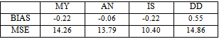
The mean bias and the mean squared error are two statistical parameters normally used for model skill evaluation[15] and they were used in this work. These indexes can be defined as:

(1)

(2)

where t= time; T = number of samples available; p= observation point; P= number of points used; sim= simulated data; obs= observed data.

3. Results and Discussion

For the analyses we used horizontal fields of hydrometeors content, namely rain water, cloud droplets, hail, graupel, snow, pristine and aggregates) integrated in a vertical column, which were compared to satellite images for each case (Figure 1). We also compared the precipitation fields provided by the model with the precipitation estimates of TRMM 3B42 (Figure 2). The highest values of hydrometeors integrated in the column can be interpreted as regions where there are thicker clouds (here we refer to the clouds optical thickness, due to higher droplet concentration) and/or large vertical development.

3.1. Squall Line: April 14, 2008

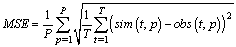
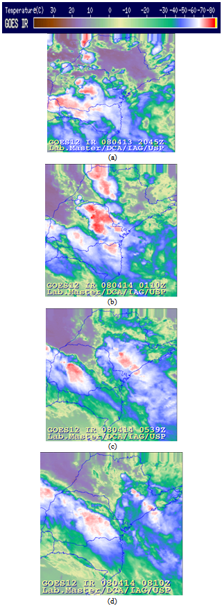
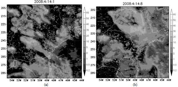
This system caused an accumulated 13.8 mm and 22.5 of rain at the INMET’s “Mirante de Santana” and “Parque do Estado” stations, respectively. An accumulation of 60 mm from 07:30 Z to 10:30 Z, obtained from the TRMM rainfall estimation, was found over MASP. We see in the satellite images a region with formation of several Squall Lines, associated with the air flow generated by a low pressure center in the South Atlantic Ocean.

This flow is responsible for transporting heat and moisture from the Pantanal region, Mato Grosso (flooded this time of year), located in the Midwest region of Brazil. Figure 2 shows the field of 3h precipitation rate obtained from TRMM. We see that there are at least two major precipitation bands caused by the Squall Line advancing from the south of the country to the southeast, passing through the MASP.

Figure 1. Satellite Images for the squal line observed during 14/04/2008, for 20:45Z (a) of 13/04/2008 and 01:10Z (b), 05:39Z (c) and 08:10Z (d) of 14/04/2008

Figure 2. Estimated 3 hours average rainfall rate (mm h-1), cantered on the time of the figure, obtained from TRMM 3B42 satellite product for 03Z (a), 06Z (b), 09Z (c) and 12Z (d) on April 14, 2008

3.2. Simulations Results

Figures 3-4 show the fields of simulated hydrometeors, these can be compared to satellite images of the case (Figure 1). In Figure 3 we see that both AN and MY options can represent well the formation of the three Squall Line that were observed in the 01Z satellite images. However, at 08Z we can see that, although both parameterizations are able to represent the Squall Line, the AN parameterization can represent the best the prefrontal Squall Line that is closer to the seacoast. IS parameterization is capable to represent the formation of some Squall Line, although their identification are not so clear. In Figure 4, DD parameterization overestimates significantly the amount of hydrometeors, but both simulations (IS and DD) have a noisy aspect, like the formation of open cumulus cells all over the grid domain.

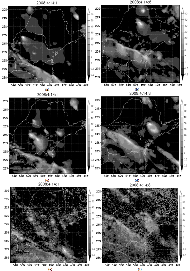Figure 3. Hydrometeors content (g kg-1) summed over all model pressure levels (1000-200 hPa) for 01Z (a, c, e), 08Z (b, d, f) of 14/04/2008 from the simulation using MY (a, b), AN (c, d) and IS (e, f) options

Figure 4. Hydrometeors content (g kg-1) summed over all model pressure levels (1000-200 hPa) for 01Z (a), 08Z (b) of 14/04/2008 from the simulation using DD options

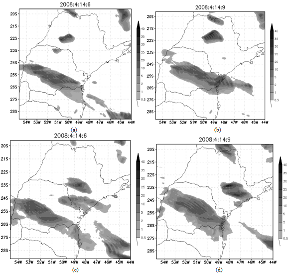Figure 5. 3-hours averaged precipitation rate (mm h-1), centered on the time of the figure obtained from the simulation with the MY (a, b) and AN (c, d) options for 06Z (a, c ) and 09Z (b, d) on April 14, 2008

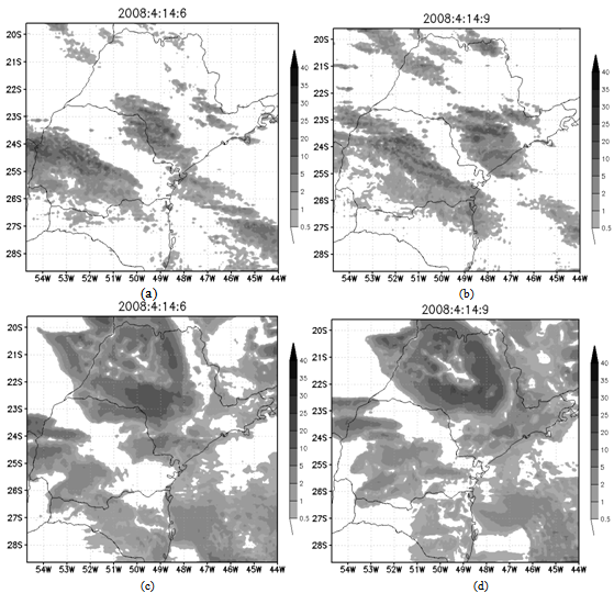Figure 6. 3-hours averaged precipitation rate (mm h-1), centered on the time of the figure obtained from the simulation with the IS (a, b) and DD (c, d) options for 06Z (a, c ) and 09Z (b, d) on April 14, 2008

At first glance, we can see a major difference between the simulations using the option MY and AN (figures 3 and 5) in comparison with the simulations using the options IS and DD (figures 3, 4 and 6). This is due to the horizontal grid spacing being much larger than the vertical one. MY and AN options are more appropriate for these cases. As pointed out by Walko et al (2007)[14], in this case it is necessary that the horizontal diffusion be stronger (for numerical dumping) than it would be on physical grounds and the model assumes total decoupling of horizontal and vertical diffusion in all aspects, including the calculation of deformation rates, length scales and components of the stress tensor.

Figures 5-6 show the 3h precipitation rates obtained from simulations, which can be compared with the precipitation rates provided by TRMM (Figure 2). The simulation using MY parameterization can represent the precipitation associated to the frontal Squall Line, failing only in the location of prefrontal system. The simulation using AN formulation can provide both frontal and prefrontal, representing fairly well the system’s location. The simulation using IS parameterization can also represent well the positioning of the Squall Line, but it fails to generate cells with pronounced rainfall rates. The simulation with DD option do not represent the precipitation observed correctly, clearly overestimating the precipitation rate.

Table 1 presents the values found for BIAS and MSE calculated for each simulation, based on the 3 hours averaged precipitation rate compared to the estimative provided by TRMM, for all simulation grid points and all time periods available at each 3 hours. (11 times used, from 15Z of April 13, 2008 up to 21Z of April 14, 2008).

Table 1. Simulation’s BIAS and MSE

We see that in general the simulations underestimate the precipitation, except DD, in which the results were overestimated. However, the bias found for the AN was very close to zero.

In calculating the MSE, the lowest values were obtained by using IS parameterization, due to the fact that this simulation does not provide high levels of precipitation and thus reduce the largest errors. However, it results in a great tendency to underestimate the simulated precipitation.

4. Conclusions

The simulation that seems to better represent the prefrontal Squall Line case was the one that used the AN parameterization option, because it can generate the observed Squall Line and its position appropriately in comparison with satellite images and also because it showed low values of BIAS with low tendency to underestimate the precipitation rates. Using the MY option, the prefrontal Squall Line location is not well represented. The simulation using IS formulation can represent the correct location of the Squall Line, but it underestimates significantly the precipitation values. The use of Deardorff parameterization was the one that provided the worst results, not being appropriate for simulations of this type of phenomena.

ACKNOWLEDGEMENTS

The authors acknowledge the financial support of CNPq and CAPES for the conclusion of this work.