1. Introduction

Major Greek cities are suffering from increased particulate emissions levels[1-4]. Volos is no exception to this fact. The city is neighboring with an important industrial area to the West and a cement factory to the East. It has a moderate traffic problem in the city center and an active commercial harbor in the southern part. It is bounded by Mount Pelion to the North. Amospheric inversion episodes are not uncommon. Since the year 2001, a significant effort has been made by the Greek Government to enhance air quality monitoring in major urban areas. A network of 28 stations was installed in 2001, mainly in Athens and Thessaloniki[4]. Volos was equipped with one monitoring station (Station O in Figure 1). The measurement of PM₁₀ in the specific family of stations is carried out by means of beta attenuation mass measurement instruments[5]. By the year 2011, Volos’ station has already completed 10 years of operation and suffers from maintenance problems. Thus, the management of particulate emissions from urban traffic, industrial activity and garbage burns in the greater urban area is limited by inexact knowledge of particulate movement and dispersal in the area as a whole, and on medium and small-topographic scales in particular.

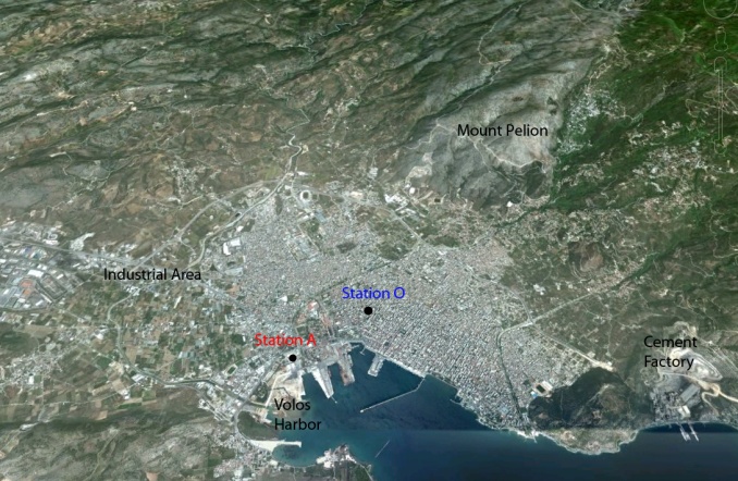Figure 1. Location of the monitoring station A at the University Campus at Pedion Areos, and the official monitoring station O at the center of Volos

In response to the above problems and the increasing civic awareness of particulate pollution problem in Volos, we started investigations with a portable instrument in 2002. This work continued in view of the Athens 2004 Olympics (Volos hosted a few Olympic activities). Following an initial assembly, testing and improvements’ period, a PM₁₀ monitoring station was established inside the University Campus at Pedion Areos in November 2004. PM₁₀ monitoring was carried out with a TSI Dusttrak 8520 instrument[6], with operation principle based on 90^o light scattering. The location is neighboring to Volos’ commercial harbor (Station A in Figure 1). The specific site for the station was selected based on its proximity to the town center and the commercial harbor. The station is located Southwest of the official measurement station (“Station O” in Figure 1).

Daily recordings and monthly summaries of PM₁₀ concentrations measured are routinely published in the Department’s website (Figures 2-3), since the beginning of 2005.

This website became popular in Volos during the winters of 2005 and 2006, when pollution episodes of several days’ duration were recorded (Figure 2). High particulate levels were correlated with atmospheric inversion during these events. Monitored PM₁₀ data were routinely compared to the data from the neighboring, official measurement station O (Figure 1). The design of the monitoring station and the selection of the measurement instrument were based on the principles of low initial and maintenance costs and good networking capabilities, to allow for future extension to a more broadly based air monitoring network for the Volos urban area that could address the above issues.

Initially the project was self-financed. The Department of Mechanical Engineering supported the project by supplying a room for hosting the station and networking facilities, as well as by hosting the web-based application in its web server. Station A initially employed a Dusttrak 8520 instrument, a simple meteorological station, a UPS and a PC with serial communication to the instrument. A Labview code was employed to perform automatic sampling of the measurement data, production of 5 minute – averages and producing the graphs of Figure 2 for online publishing as a web page, (www.pm10.uth.gr). Monthly reports of the hourly variation of PM₁₀ concentrations are automatically compiled and published in the same website, as monthly bulletins in the form of Figure 3. The provision of real-time air quality data was selected to assist with the management of ambient particulate concentration, being a valuable public awareness tool. The station operates year-round and people are expected to supply information on visual observations, when they spot any important particulate emissions events. Since January 2010, the monitoring instrument was updated to the Dusttrak II 8530[7] which includes an Ethernet communications link. This allows easier extension to a network of instruments that may be polled by a single computer[8].

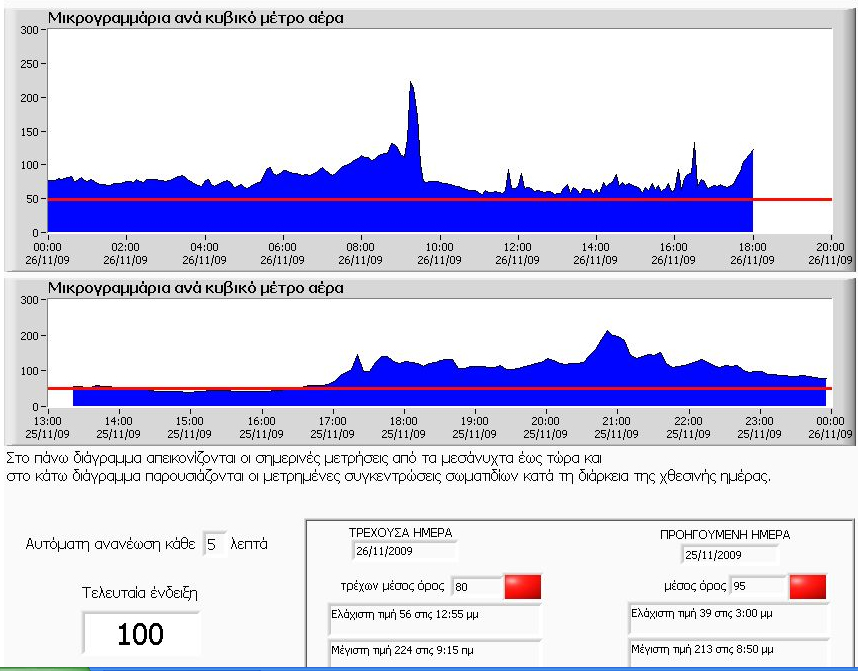Figure 2. A screenshot of the web based PM10 monitoring (episode of 25/11/2009). PM10 variation during the current/ previous day is depicted in the upper/ lower graph respectively. Last measurement, PM10 mean, maximum and minimum values are also presented for both days

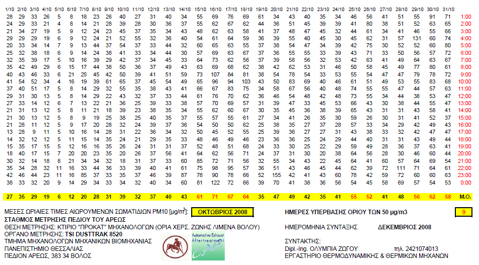Figure 3. Typical structure of a monthly PM10 bulletin as published in the website (October 2008). Hourly PM10 means for the 24 hours of the respective day are presented in each column

After 5 years of systematic PM₁₀ monitoring in the site, a substantial amount of data were compiled that was subjected to statistical analysis, correlation with meteorological data and comparison with the recordings of the official monitoring station, aiming to assess the feasibility of PM₁₀ monitoring in urban areas employing low cost measuring equipment. The details and results are presented below.

2. Measurement Instruments and Monitoring System

Based on an initial instrument survey, it was realized that a continuous reference instrument, such as a Tapered Element Oscillating Microbalance (TEOM) or Beta Attenuation Mass measurement (BAM) instrument, would be likely to require a substantial expenditure on supporting infrastructure (e.g. air conditioned enclosure etc), and significant power and maintenance resources, while providing only hourly time resolution[9]. In contrast, previous experience with an optical particle counter (TSI 8520 DustTrak) had shown that a relatively low-cost instrument could give a very good proxy measurement of PM₁₀. This is confirmed by experience from other researchers_[10, 11].

In order for the station and the future network to operate successfully, it was considered necessary to be equipped with an air quality instrument capable of continuous measurement, (preferably subhourly time resolution). The equipment had to be securely housed and to require only basic maintenance to operate under automatic control for long intervals. Low total power consumption and a small footprint were considered significant advantages. The overall cost needed to be as low as possible.

Data collected with such an optical instrument are not mass measurements, but are a proxy based on a measured particle count and a calibration from counts to mass for the particular aerosol under study. Optical particle counters tend to be more sensitive to smaller particle, due to the nature of light scattering from aerosols[12].

Several optical particle counters are commercially available[9]. Dusttrak II 8530[7] is a network enabled device, providing a simple and direct means of communicating with the instrument remotely. The instrument provides estimates of PM1, PM2.5, PM4, and PM10, depending on which diffuser is inserted. The device can be field calibrated by the operator.

One possible confounding signal that arises when using optical scattering methods is the presence of high-humidity in the sample air, with the most extreme case being fog. Scatter from water droplets can mimic that from smoke or other aerosols, hence optical measurements taken under these conditions can overestimate the true PM signal[13]. Early experience with the model 8520 DustTrak showed this effect. The Beta Attenuation Mass Measurement instruments are also sensitive to relative humidity. To overcome this effect, the air being passed to the instrument can be preheated by drawing the sample air through a heated tube.

A suitable meteorological station was also required. A variety of such stations are commercially available, with a corresponding wide range of costs. While there were advantages in using a ‘high-end’ meteorological station, it was decided that, given the air quality data would be ‘indicative’ rather than reference-quality data, there were significant cost advantages in selecting a basic meteorological installation. The Global Water GL400 data-logging weather station was chosen after a comparison of available systems. Labview was used to provide on-board data storage and network IP communications.

Network communications to the station was an issue of active consideration. The older model Dusttrak 8520 was communicating with a networked PC via serial port. The more recent model Dusttrak II 8530 is equipped with an Ethernet communication (LAN) port. The instrument is given a fixed IP address within the University firewall.

The inlet of the sample line exits the station wall at a height of 3m from ground, and is turned in a gentle curve to point downwards. It is protected from insects’ ingress by a fine wire mesh.

Labview was employed for communication, data reporting and analysis, and web publication. A custom made code is written to this purpose. Communication with the instrument at a given station is via calls to an internet SOCKET command[8]. The code routinely polls one or more stations and receives second-by-second readings from the Dusttrak instruments. Also, it receives recordings from the meteorological station, via serial port communication. The PC running the program is located in the main station A, connected by serial communications cable to the met station. All data from the network are retrieved via this PC. Labview also provides the tool for creating the graphical user interface for the web publishing.

Data from the Dusttrak and meteorological instruments are written to a daily file. A plot of these data is generated and displayed on the data-logging PC. The plot files are also written to the server disk after each data read, and copied to a web server for public viewing.

More details on the comparative performance of the two types of instruments are presented in a subsequent section. As regards the quality assurance of the collected data, the following basic steps are taken (see for example[14]):

● Elimination of outliers in the measured data (unmeasured values, erroneous values, negative values etc), caused by instantaneous failure of the instrument or data logging system. The missing values are substituted by values interpolated from neighboring values.

● Basic FFT analysis of the measurement signals, to bring into the foreground the most important periodicities in each measured variable. Again, the existence of very high frequencies in immisions points to instrument or data logging failure, or the presence of temporary sources of local nature in the vicinity of the station. Such sources may damage the quality of the measured data sets.

● Signal filtering by low pass finite impulse response (FIR) filters that eliminates the above-mentioned noise and leads to smoother measured data time series.

Following the processing of data by the above methodology, we now proceed to the presentation of final, corrected data time series and their basic statistics.

3. Overview of the Measurement Data

The adoption of the new Directive 2008/50/EC[15] on ambient air quality and cleaner air for Europe signals the merging of most of existing legislation into a single directive (except for the fourth daughter directive) with no change to existing air quality objectives. Thus, the limit of 35 days of exceeding the 50 μg/m³ threshold in PM₁₀ from the previous Directive 1999/30/EC[16] remains in force, along with the 40 μg/m³ limit in the annual PM₁₀ mean value. In addition, new air quality objectives are introduced for PM_2.5 (fine particles) including the limit value and exposure related objectives – exposure concentration obligation and exposure reduction target. Also, it introduces the possibility to discount natural sources of pollution when assessing compliance against limit values. A possibility for time extensions of three years for PM₁₀ for complying with limit values is also included, based on conditions and the assessment by the European Commission. More stringent requirements including a 28 μg/m³ limit in the annual PM₁₀ mean value and a 24-hour limit of 35 μg/m³ not to be exceeded more than 35 days annually are introduced starting 2010.

The evolution of annual PM₁₀ levels and number of days exceeding the 50 μg/m³ threshold, as measured by the two monitoring stations of Figure 1, are presented in Figure 4 for the period 2002-2010. The following remarks can be made here:

High levels of yearly average ambient PM₁₀ concentrations, significantly exceeding the 40 μg/m³ limit of the directive, persisted in Volos in the period 2002 to 2006. These high PM₁₀ levels were accompanied with a large number of days exceeding the 50 μg/m³ threshold – more than 100 days each year[17].

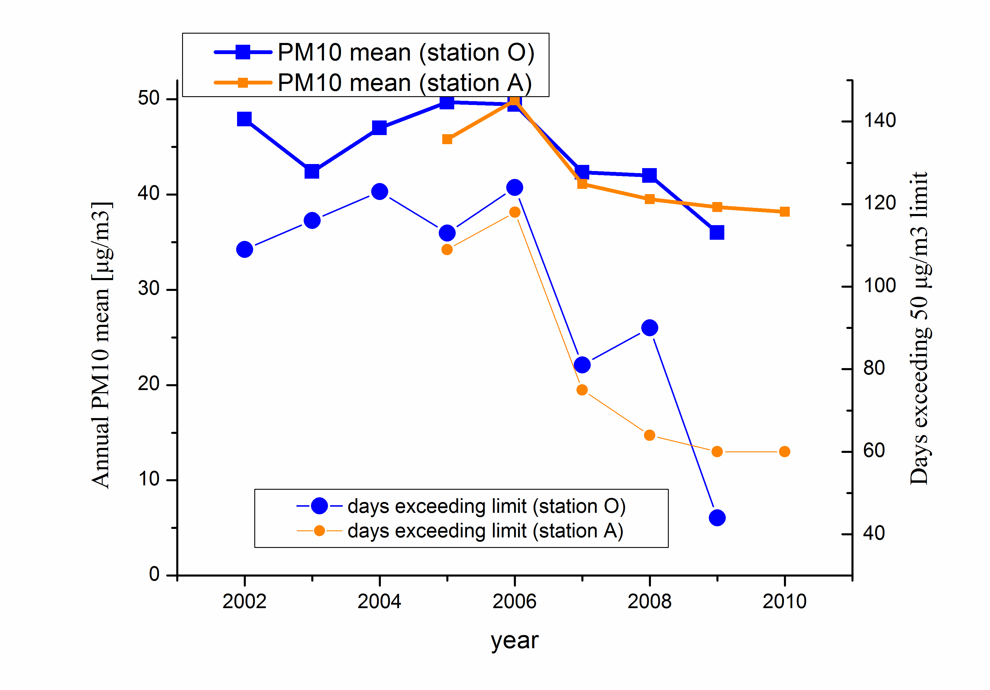Figure 4. Evolution of annual PM10 concentrations and number of days exceeding the 50 μg/m3 limit in the town of Volos since 2002, as measured by the Official station (station O) and the University station (station A), respectively

Starting from 2007, we observe a significant reduction trend for the annual average PM₁₀ levels with a tendency to stay below the 40 μg/m³ limit after 2008, along with a reduction in the number of days exceeding the 50 μg/m³ threshold, with a tendency to stabilize at about 60 days.

As regards the comparative measurement data from stations O and A, one could observe that there existed a good overall agreement during the years 2005, 2006 and 2007. Towards the second half of 2008 we observed that station O reported significantly higher number of days exceeding the 50 μg/m³ threshold, which cannot be easily explained. One must take into account in this respect that the beta attenuation instrument of station O is already 10 years old, and the station ceased to report data towards the end of 2010. Having this in mind, we are going to limit accordingly our period of performance comparison between the two instruments.

The reduction in ambient PM10 levels since 2007 is a fact that was observable to the citizens of Volos and could be correlated with the following facts:

● A significant reduction in industrial production of major local industries, since the end of 2007, due to economic recession and a significant reduction in local industrial production activity.

● The gradual introduction of natural gas for space heating in the residential sector which started in 2002 and its growth rates peaked in 2007.

● The significant reduction of the average age of the vehicle fleet in Greece (and Volos) that was observed in the period 2002-2008.

Following this overall assessment of the measured data sets and the quality of ambient air regarding particulate matter in the period of interest, we proceed to analyse the available hourly or 5-minute data, against existing meteorological data, aiming at drawing useful conclusions on the effect of the micro-climate and the feasibility of low-cost particle levels monitoring and the possibility of spotting important factors affecting the PM₁₀ levels.

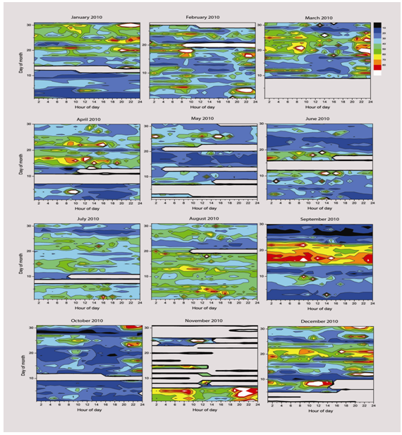Figure 5. Summary of station A hourly measurements during the 12 months of 2010 in Volos. Grey areas indicate lack of data due to instrument problem. White areas denote PM10 values exceeding 90 μg/m3

As a first step, it would be interesting to see an overall picture of the hourly PM₁₀ levels for a full year, as measured by station A during 2010 (Figure 5). Each month is presented in a separate graph. A color code is applied, with brighter colors associated with higher PM₁₀ levels. Yellow, orange, red and finally white color corresponds to levels exceeding 60 μg/m³. Each separate graph is made up of 28, 30 or 31 horizontal strips, according to the respective number of days in the month. In this way, one can observe looking vertically, if high PM₁₀ levels are associated with a specific time-belt in the day. For example, we observe persisting, significant PM₁₀ measurement levels during hours 20:00-24:00, in a large number of days in October, November, December, January, February and March. This should be associated with the operation of fossil fuel heating equipment and especially wood stoves, as well as increased cold start emissions of engines during winter[2]. Another daily time belt that is associated with significant PM₁₀ peaks is the one from 08:00-16:00. As regards the above observations, it should be additionally mentioned that station A is affected by Volos Harbor activity, as well as the (limited) traffic inside the University Campus. The PM₁₀ measurement increase during the evening could be further correlated to the micro-climate as mentioned in a subsequent section. Analogous patterns of temporal variation on a seasonal and a daily base is also reported by other researchers[18].

4. Comparisons of Recordings from Two Different Instruments

As already mentioned, there exists one further issue with PM₁₀ monitoring, where the statistical analysis may ensure favorable conditions for the exploitation of low-cost measuring equipment, to give a very good indicative (proxy) measurement of PM₁₀. Correlation of recordings from the two different instruments, adding to the experience from the study and statistical analysis of recordings from the Dusttrak and beta attenuation instruments has already been reported by other researchers[19].

A comparison of the recordings from the Dusttrak 8520 instruments in station A to those of the beta attenuation instrument in station O may give us useful information, although the two instruments have different operation principles, and their locations are at a distance of about 1 km (see Figure 1).

During the period 2005-2008 the 24-hour averages of the two monitoring stations generally show a good overall agreement as seen in the example of Figure 6 (May 2008).

Obviously, the 24-hour means agree to a certain degree. To a good approximation, the proxy PM₁₀ values, derived from the 24-hour-averaged DustTrak reading, gives a reliable measure of PM₁₀. These data were in fact used in 2005 to check the calibration of the DustTrak 8520 instrument, based on the data from the beta attenuation measurement instrument. Of course, the two stations are in different locations, so they are not expected to give similar results on an hourly basis. Anyway, it would be interesting to compare the transient recordings from the two stations. This is shown in the comparison between recordings of Stations O and A in Figure 7, where data from both stations for the period May 2008 are shown. A qualitative agreement is only observed in this case.

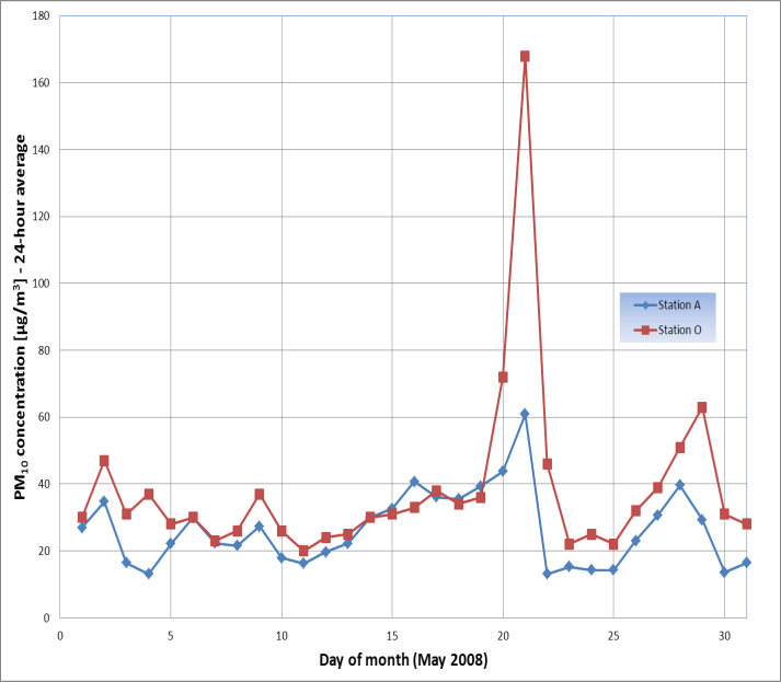Figure 6. Comparison between 24-h average PM10 concentrations recorded at station A (Dusttrak 8520) and station O (beta attenuation instrument) recordings during May 2008

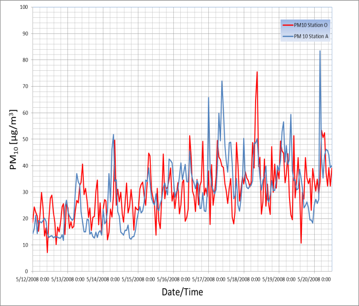Figure 7. Comparison of hourly PM10 recordings of Dusttrak 8520 in station A to recordings from the beta attenuation instrument in station O location, during the period 12-20 May 2008

This is expected since the location of the two instruments is not the same: Dusttrak 8520 was located at station A, at the periphery of the University Campus, whereas the beta attenuation instrument was located at station O, in the city center. For example several peaks observed in station A recordings in Figure 7 are readily correlated with emissions from heavy Diesel vehicles operating in the neighboring Volos’ harbor zone.

5. Correlation of PM10 Concentration with Meteorological Conditions

Having confirmed a good correlation of the readings from the two stations, we proceed to investigate the effect of the following meteorological data to the PM₁₀ levels:

Wind direction, wind speed, ambient dry-bulb temperature, absolute and relative humidity.

As a starting point, it is interesting to observe the evolution of meteorological conditions and PM₁₀ emissions in station A during one full week of May 2010, as presented in Figure 8. The specific week was selected to be free from significant activity of residential heating equipment in the city. A number of interesting remarks can be made here:

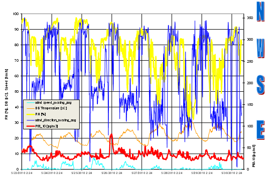Figure 8. Evolution of meteorological conditions and PM10 emissions in station A during one full week of May 2010

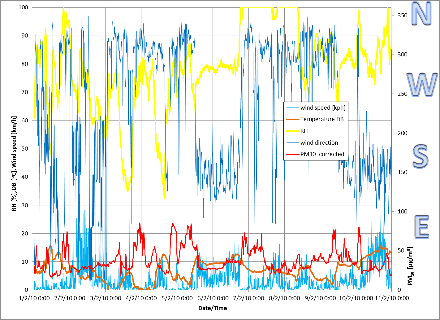Figure 9. Meteorological conditions and PM10 emissions in station A during 11 days of February, 2010

This week of spring is characterized from the absence of abrupt weather changes and the absence of precipitation (which would clean the air). Thus, the local wind system and micro-climate is clearly observable. This figure clearly presents the repeating daily pattern of the sea breeze (South to South-East wind direction with a maximum wind speed of 5-8 km/h, higher air temperature and lower relative humidity) during the late morning- to- noon hours, followed by the land breeze (North-West wind direction with very low wind speed, lower air temperature and higher relative humidity) during the late night. Obviously, the sea breeze brings low particulate levels, whereas the land breeze brings higher particulate levels from the urban interior. Also, Northeastern and Eastern wind is associated with high particulate levels in several instances in this figure. These effects are very clearly observable. As regards the effect of relative humidity, it should be mentioned that the warm sea breeze has a lower relative humidity than the cold land breeze of the night.

Further, it is also interesting to see the respective behavior recorded by station A, during a typical winter month with windy and low temperature weather conditions (February 2010). This is presented in Figure 9. The operation schedule of the residential heating equipment is clearly observable in this figure from its effect on the particulate levels, which become more intense as ambient temperatures go below zero.

The following remarks can be drawn on this figure: Southern winds always reduce the particulate levels in station A. Low wind speeds are associated with high particulate levels, especially when the wind direction is from the Northwest (which is the direction of the Industrial Area, as well as the urban area of Nea Ionia). Eastern wind is also associated with higher particulate levels in some instances in this figure.

Following these first-hand observations, it would be interesting to see whether statistical analysis of the PM₁₀ data based on the meteorological data for the specific site, would confirm the above or point to additional effects[20]. Commercial software is employed for statistical analysis[21]. One-way ANOVA is employed to check the effect of the wind direction, wind speed, ambient temperature, Relative Humidity and Humidity ratio on the PM₁₀ concentration levels[22]. Once a statistically significant dependence is confirmed, the prevailing PM₁₀ levels in each category are plotted. The exact way of defining the classes for each variable is presented in Table 1.

5.1. Effect of the Hour of day

A one-way ANOVA applied to the hourly PM10 values of the year 2010, versus the variable “hour of day” gives the results presented in Table 2.

As expected from everyday experience, the PM₁₀ concentrations are dependent on the hour of day with a good reliability (F=81) and Significance = 0.000.

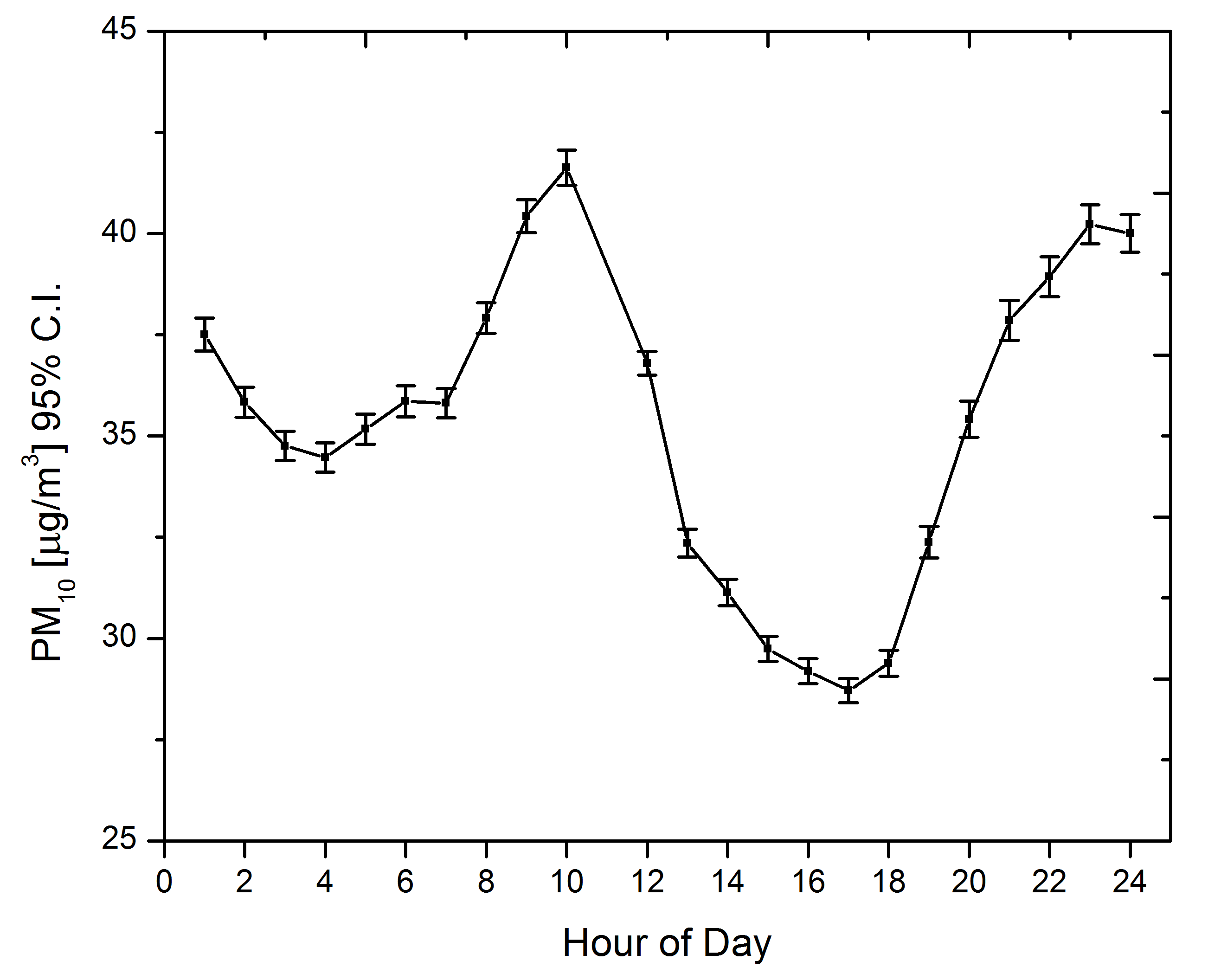Figure 10. Standard error of mean of PM10 concentration versus hour of day

Now, the statistical evolution of mean PM₁₀ concentration in the 24 classes corresponding to the hour of day can be presented in Figure 10 along with its standard error of mean (±2σ). Again, the observed peak at 09:00-10:00 in the morning should correspond to local traffic in the campus from incoming students’ and faculty private cars, along with increasing commercial harbor traffic. The observed valley with low PM₁₀ concentrations during the noon hours could be related to the cleansing effect of the sea breeze explained in the context of Figure 8. Similar daily patterns are reported by other researchers in urban areas[23].

Table 1. Selection of class intervals for the main independent variables examined Class Variable 1 2 3 4 5 6 7 8 Wind direction 0-45 45-90 90-135 135-180 180-225 225-270 270-315 315-360 Wind speed ≤1 1-5 6-11 12-19 20-28 29-38 39-49 ≥50 Ambient DB temperature ≤0 0 - 5 5-10 10-15 15-20 20-25 25-30 >30 Ambient Rel. Humidity 0-20 20-40 40-50 50-60 60-70 70-80 80-90 90-100 Ambient Humidity ratio ≤0.003 0.003-0.006 0.006-0.009 0.009-0.011 0.011-0.014 0.014-0.017 0.017-0.020 >0.020

Table 2. Results of one-way ANOVA applied to the hourly PM10 values of 2010, versus “hour of day” Sum of Squares df Mean Square F Sig. Between Groups 590837.216 22 26856.237 81.805 .000 Within Groups 1.566E7 47712 328.298 Total 1.625E7 47734

Table 3. Results of one-way ANOVA applied to the hourly PM10 values of 2010, versus “DB Temperature” Sum of Squares df Mean Square F Sig. Between Groups 927636.656 7 132519.522 412.656 .000 Within Groups 1.533E7 47727 321.138 Total 1.625E7 47734

Table 4. Results of one-way ANOVA applied to the hourly PM10 values of 2010, versus “Relative Humidity”. Sum of Squares df Mean Square F Sig. Between Groups 1072198.037 6 178699.673 561.768 .000 Within Groups 1.518E7 47728 318.102 Total 1.625E7 47734

5.2. Effect of ambient Temperature (DB)

A one-way ANOVA applied to the hourly PM10 values of 2010, versus “Dry bulb temperature” gives the results of Table 3.

Thus, PM₁₀ concentrations are dependent on ambient temperature levels with high reliability (F=412). Significance is again 0.000

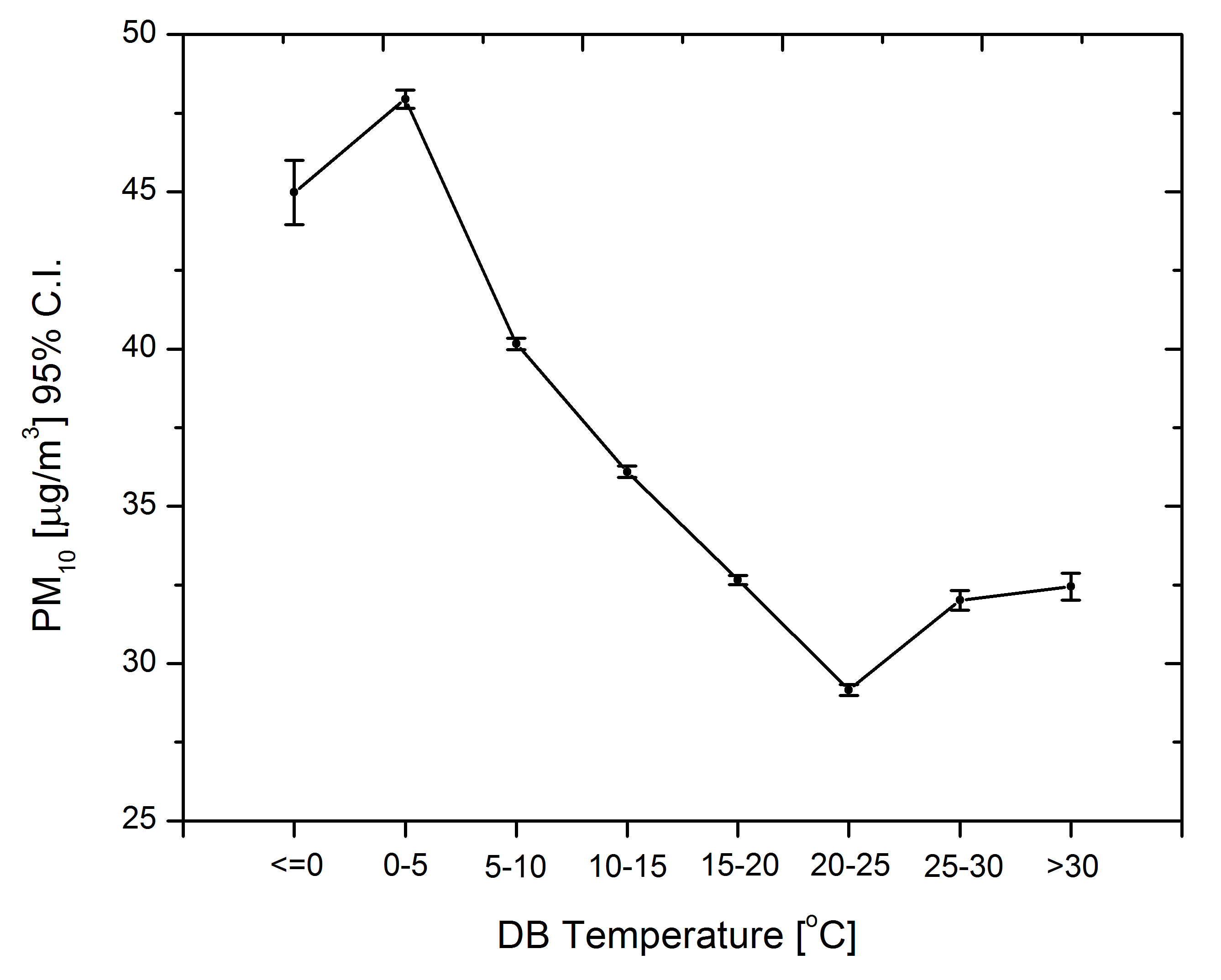Figure 11. Standard error of mean of PM10 concentration versus ambient temperature

Based on this confirmed significant effect, it is interesting to look at the statistical evolution of mean PM₁₀ concentration in the 8 temperature classes of Table 1, as presented in Figure 10.

A number of observations can be done here: First, low ambient temperatures are associated with higher average particulate levels and this should be clearly related to the operation of residential heating devices as already mentioned above. The minimum average levels of PM₁₀ are observed in the ambient temperatures’ class between 20-25^oC, which clearly agrees with the human thermal comfort temperature zone.

A certain increase in PM₁₀ concentration is statistically significant at higher ambient temperatures. This may be due to the enhanced photochemical activity during days with increased solar intensity[24]. It should be additionally noted in this respect that ambient temperature is not completely independent from the remaining weather variables.

6. Effect of Relative Humidity

A one-way ANOVA applied to the hourly PM10 values of 2010, versus “Relative Humidity” gives the results of Table 4.

Thus, the PM₁₀ concentrations are dependent on the relative humidity with high F (F=561).

The strong effect of the relative humidity on the PM₁₀ levels can be explained based on the following factors: (i) high relative humidity is usually associated with low wind speed and temperature inversion episodes, (ii) very low relative humidity is associated with a dry, dusty urban atmosphere and (iii) the operation principle of the specific type of instrument makes it more sensitive at close-to-saturation conditions, which forms the main weak point of the specific type of instrument[19].

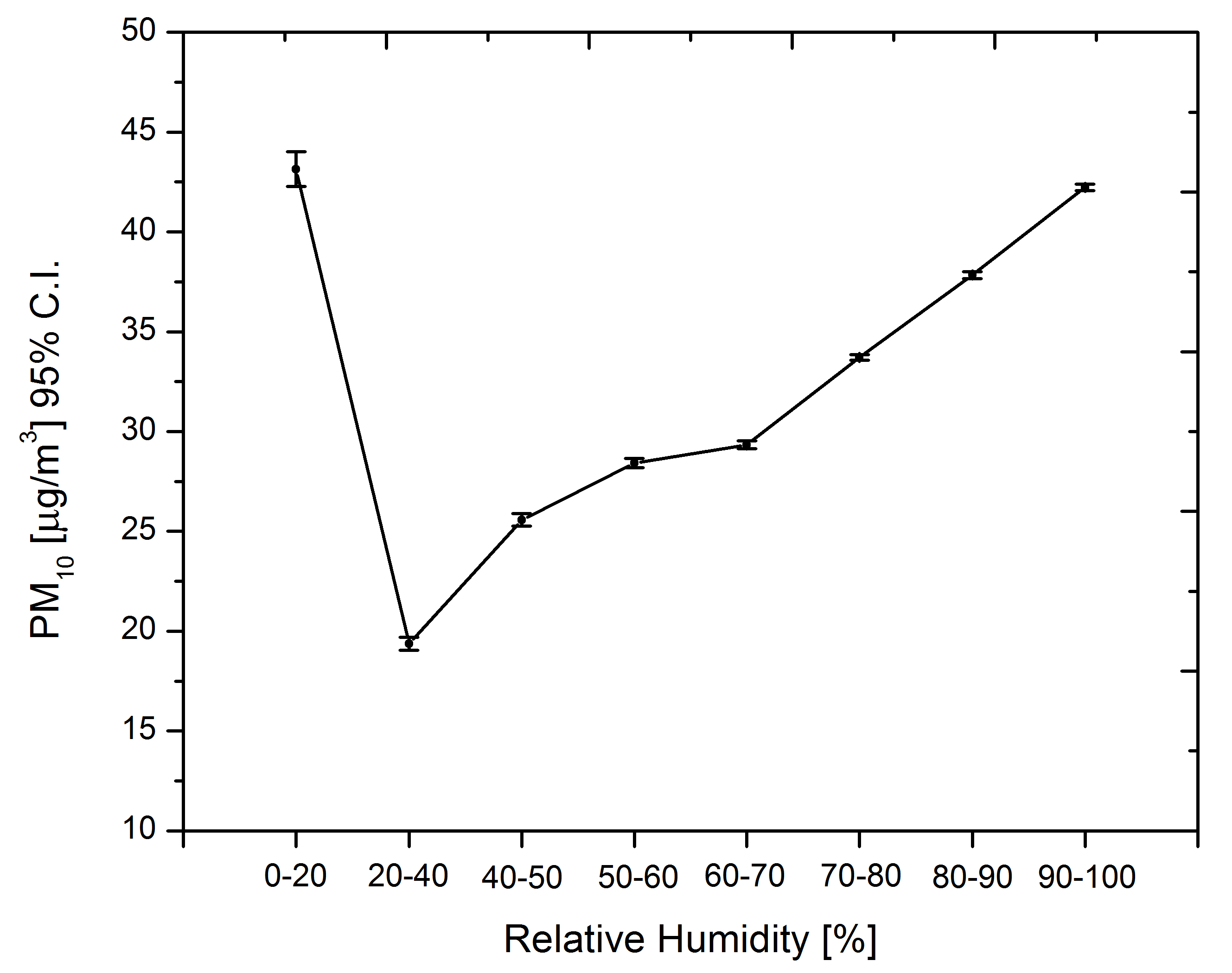Figure 12. Standard error of mean of PM10 concentration versus relative humidity

Based on the confirmed good statistical correlation of PM₁₀ levels to relative humidity, it would be interesting to look at the statistical evolution of mean PM₁₀ concentration in the 8 relative humidity classes of Table 1, as presented in Figure 12. High relative humidity levels are shown to be associated with high PM₁₀ levels, and the same is true for extremely low relative humidity levels.

Further investigation would be interesting regarding the correlation between relative humidity and measured PM10 as being due to the presence of sea-salt aerosols (whose growth rate depends on relative humidity)[13].

Further, it is interesting to investigate the effect of alternatively placing the humidity ratio as independent variable. F is again high, indicating a statistically reliable effect.

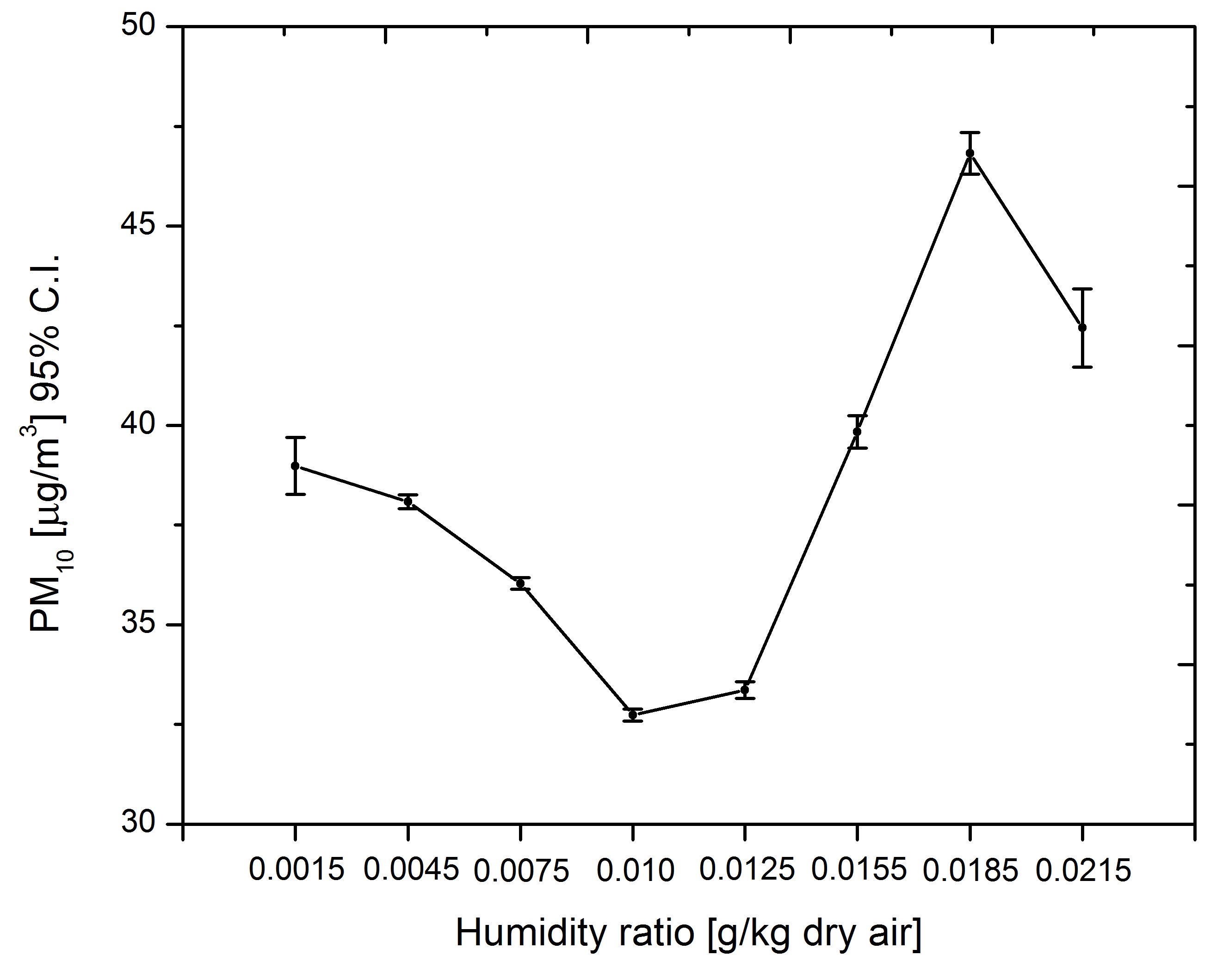Figure 13. Standard error of mean of PM10 concentration versus humidity ratio of ambient air

The statistical evolution of mean PM₁₀ concentration in the 8 humidity ratio classes of Table 1, is presented in Figure 13.

The same overall statistical dependence is observed here, if one keeps in mind the strong correlation of the various class intervals with ambient temperature (for example, classes 1,2 and 3 are associated with very low temperatures in the specific micro-climate).

7. Effect of Wind Direction

A one-way ANOVA applied to the hourly PM₁₀ values of the year 2010, versus the variable “wind direction” gives the results presented in Table 5.

Thus, PM₁₀ concentrations are dependent on the wind direction with a good reliability (F=149 and Significance =0.0). This statistical analysis result agrees with what is known from everyday experience and what is mentioned in the literature.

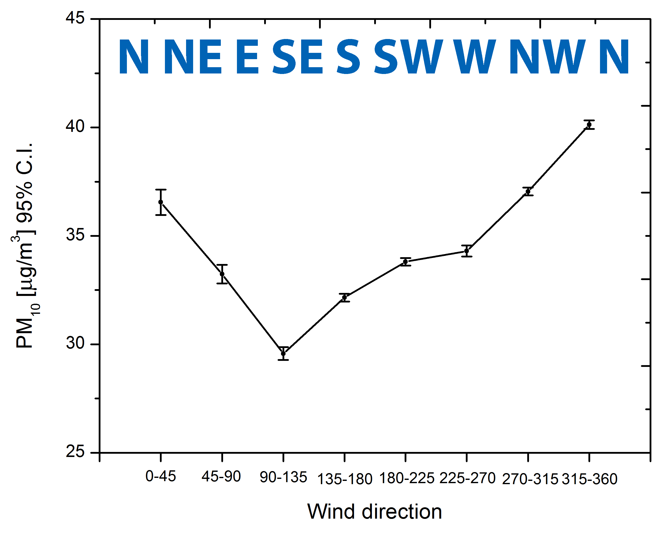Figure 14. Standard error of mean of PM10 concentration versus wind direction

Based on this confirmed, good statistical correlation of PM₁₀ levels with wind direction, it is interesting to look at the statistical dependence of mean PM₁₀ concentration in the 8 wind direction classes of Table 1. The corresponding wind directions are depicted at the top of the graph to allow a better understanding of the figure. The already mentioned association of W, NW, N and NE winds to high PM₁₀ levels is also implied here (see Figure 1). Statistically, the lowest PM₁₀ levels are associated with South-East winds from the sea (Pagasitikos Gulf), as already seen in Figures 8 and 9.

8. Effect of Wind Speed

A one-way ANOVA applied to the hourly PM₁₀ values of the year 2010, versus the variable “wind speed” gives the results presented in Table 6.

Apparently, the PM₁₀ concentrations are dependent on the wind speed with a good reliability (F=247 and Significance =0.0). Again, this result agrees with everyday experience and what is reported in the literature.

Table 5. Results of one-way ANOVA applied to the hourly PM10 values of 2010, versus “Wind Direction” Sum of Squares df Mean Square F Sig. Between Groups 349882.628 7 49983.233 149.990 .000 Within Groups 1.590E7 47727 333.243 Total 1.625E7 47734

Table 6. Results of one-way ANOVA applied to the hourly PM10 values of 2010, versus “Wind speed”. Sum of Squares df Mean Square F Sig. Between Groups 490133.561 6 81688.927 247.319 .000 Within Groups 1.576E7 47728 330.298 Total 1.625E7 47734

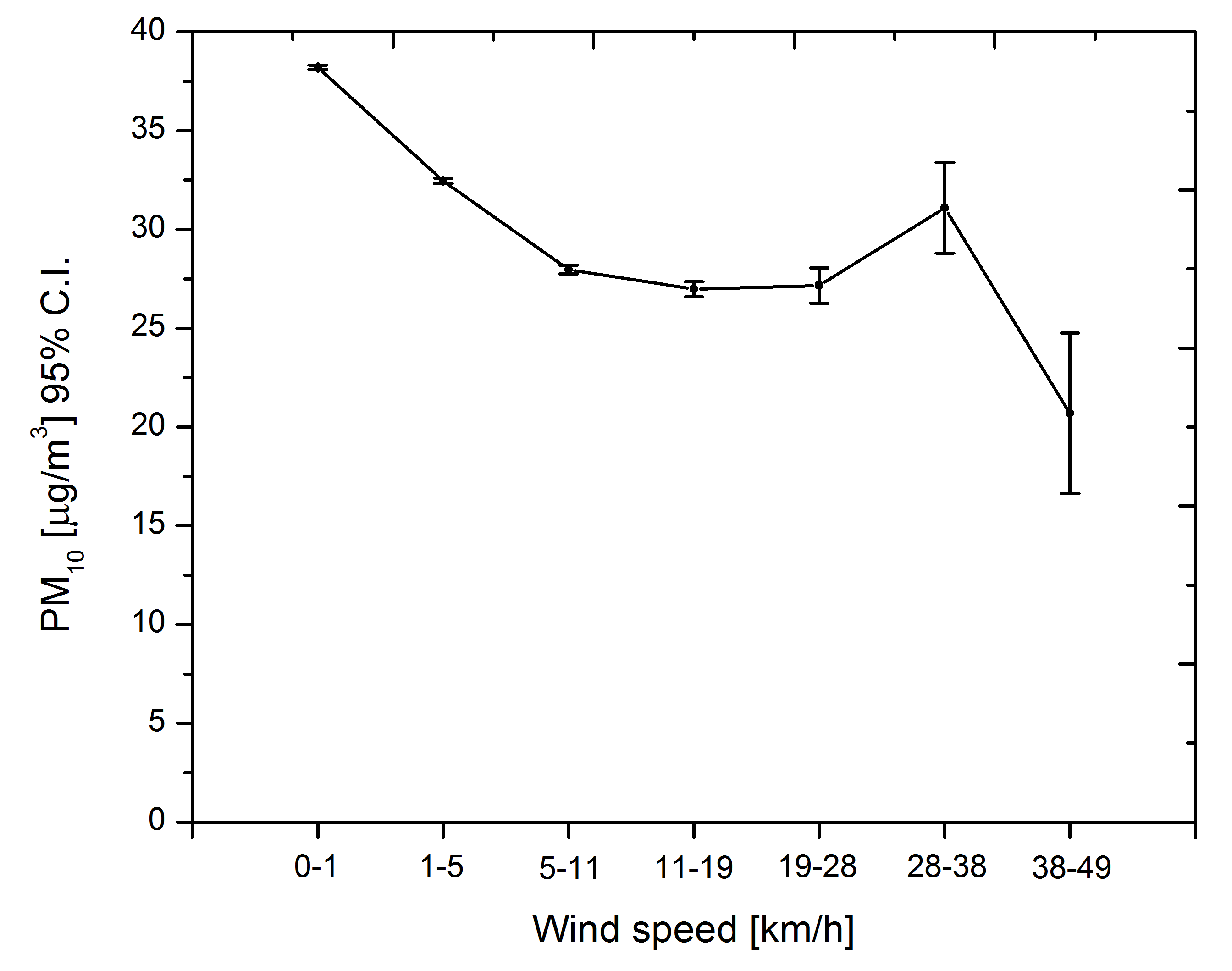Figure 15. Standard error of mean of PM10 concentration versus wind speed

Based on this confirmed, good statistical correlation of PM₁₀ levels with wind speed, it is interesting to look at the statistical dependence of mean PM₁₀ concentration in the 8 wind speed classes of Table 1 (which correspond to the Beaufort scale). Stronger winds are shown to be statistically associated with lower PM₁₀ levels, up to a speed of about 30 km/h, beyond which the situation reverses, albeit with a much wider statistical confidence interval. The inverse correlation of PM₁₀ levels with wind speed is also reported by other researchers[1, 24].

Summarizing, the dependence of measured PM₁₀ on the following weather variables is proven with high reliability: Relative Humidity, ambient temperature (DB), wind speed, wind direction. The same is true for the dependence on the hour of day. Table 2 summarizes the respective F values resulting from the statistical analysis of the 2009 and 2010 PM₁₀ data.

In addition, this table presents, for comparison, the respective F values resulting from statistical analysis of the full two-year set of PM₁₀ data. It should be observed that the quantitative results for 2009 and 2010 are matching very well, which is an additional check for the validity of analysis.

As a general observation, we get a steady zero significance for all ANOVA cases, despite the fact that in several variables (as for example, the hour of day), the standard deviations do not differ at least from a first glance.

Table 7. Comparison of F values for one-way ANOVA of PM10 concentration with respect to several weather variables and the hour of day, as applied to the 2010 data, the 2009 data and the full set of 2009/2010 data Independent variable F value (2010 data) F value (2009 data) F value (2009-2010 data) Relative Humidity 562 521 875 ambient temperature (DB) 413 530 557 wind speed 247 97 364 wind direction 150 91 212 hour of day 82 29 96

As a next step, one can shift to two-way ANOVA, to assess the combined effect of DB temperature and relative humidity to PM₁₀, which results in strong dependence of PM₁₀ from relative humidity, a weaker dependence from ambient DB temperature and a dependence of PM₁₀ from the combined effect of high temperature – high relative humidity which are – obviously – not mutually independent variables.

Based on the experience from operation of the low-cost PM₁₀ monitoring station in the period 2005-2010, the University of Thessaly Research Committee funded the extension to a network of 3 PM₁₀ monitoring stations that covers most of the greater Volos area, with additional stations in two University buildings, East and West of the urban center, thus allowing better understanding of particulate movement and dispersal in the greater Volos urban area. The operation of this network will supply more data to support more elaborate statistical analysis and correlations and better understand the origins of particulate pollution in the city.

9. Conclusions

After 5 years of systematic PM₁₀ monitoring in Volos with a low-cost, light scattering measurement instrument, we conducted statistical analysis of the PM₁₀ measurements, correlation with the respective meteorological data and comparison with PM₁₀ recordings from the official monitoring station.

An overview of the evolution of particulate pollution in Volos was presented, indicating a significant reduction trend for the annual average PM₁₀ levels since 2007, with a tendency to stay below the 40 μg/m³ limit, along with a reduction in the number of days exceeding the 50 μg/m³ threshold, with a tendency to stabilize below 60 days/ year.

The effects of the micro-climate of the site on the PM₁₀ concentration levels are clearly visible in the analysis of recordings during the neutral season (May or October), where space heating or -cooling is not necessary.

Statistical processing of the 2009-2010 measurement data indicates a negative correlation of PM₁₀ with ambient air temperature during the heating period, and a strong positive correlation with relative humidity at high humidity levels. This last effect is related to an already known instrument sensitivity to high humidity levels.

As regards the wind direction, low PM₁₀ concentrations are associated with E to SE winds (coming from the sea) and high concentrations with NW to N winds (coming through the urban area). A negative correlation with wind speed is also observed at low-to-moderate wind speeds.

Daily variation of particulate matter concentrations follows well established patterns with peaks at 09:00-10:00 and 23:00-24:00.

The results indicate the feasibility of monitoring particulate emissions in urban areas employing low cost equipment, provided that the measured data are routinely checked by standard statistical methods. The operation of an expanded PM₁₀ monitoring network is under way.

Nomenclature

BAM→ Beta Attenuation Mass measurement

DB→ Dry Bulb Temperature

FFT →Fast Fourier Transform

FIR→ finite impulse response

PM→ Particulate Matter

TEOM→ Tapered Element Oscillating Microbalance

ACKNOWLEDGEMENTS

It is a pleasure to acknowledge the cooperation of our colleagues and collaborators, Assoc. Prof. Herricos Stapountzis, Dr. George Konstantas, Dipl.-Ing. Dimitris Tziourtzioumis, Dipl.-Ing. Loucas Dimitriades and Assist. Prof. Dimitrios Pandelis, who contributed at various stages of the PM₁₀ monitoring project in Volos in the period 2003-today.