1. Introduction

The Sun is the source of the energy that causes the motion of the compact atmosphere and thereby controls weather and climate. Any change in the energy from the Sun received at the Earth's surface will therefore affect climate. During stable conditions there has to be a balance between the energy received from the sun and the energy that the Earth radiates back into space. This energy is mainly radiated in the form of long wave radiation corresponding to the mean temperature of the Earth. Global surface temperature (GST) is a critical measure of climate variations.

A clear warming trend in the global climate, of about 0.8 ± 0.18 ºC, is observed in the last 150 yr in the global surface air temperature. A large part of this warming is attributed to the anthropogenic effects due to the enhanced green house gases concentrations[1,2 ]. Nevertheless , there seems to be some evidence that solar variability can contribute at least to part of this global warming[3–9]. The 11-yr-solar cycle and the associated variability that it has on the electromagnetic environment of Earth have been largely studied in the last decades[10,11] .

Global warming is a term used to describe an increase over time of the average temperature of the Earth's atmosphere and oceans. It has been the major variable in the ongoingpublic debate concerning the role of man-made climate change.

The observations of the global warming of the Earth since the beginning of the 20th century have been employed to infer that increased concentration of greenhouse gases are the cause. Naturally, this leads to the question of whether or not the Sun is playing an active role in this temperature rise.

Indices of geomagnetic disturbances measure the response of energetic solar eruptions that actually affect the Earth. Geomagnetic activity aa seems to be the possible link through which the solar activity controls the Earth's climate[12] . Near-Earth variations in the solar wind, measured by the aa geomagnetic activity index, have displayed good correlations with global temperature[12,13] . The total magnetic flux, leaving the Sun and driven by the solar wind, has risen by a factor 2.3 since 1901, leading to the global temperature has increased by 0.5º C. In addition, the solar energetic eruptions, which dragged out or/and organized by the observed variations in the solar wind, are closely correlated with the near-Earth environment[14,15].

On the other hand, there are many other parameters that effect on the global surface temperature upon global temperature changes have also been the concern of researchers[16,17] presented a correlative study of the possible contributions for the two solar and geomagnetic activities components (aa and Kp) , and the sunspot numbers Rz that may be closely associated with the climate, throughout the last 128 years (1880–2008).

The global Kp index is obtained as the mean value of the disturbance levels in the two horizontal field components, observed at 13 selected, subauroral stations. The name Kp originates from "planetarische Kennziffer" (= planetary index). K variations are all irregular disturbances of the geomagnetic field caused by solar particle radiation within the 3-h interval concerned. All other regular and irregular disturbances are non K variations. Geomagnetic activity is the occurrence of K variations.

The aa geomagnetic index is a simple global index of magnetic activity that is produced from the K indices of two nearly antipodal magnetic observatories in England and Australia. This index is the 3-hourly equivalent amplitude antipodal index.

Sunspot numbers (Rz)are temporary phenomena on the surface of the Sun (the photosphere) that appear visibly as dark spots compared to surrounding regions with a diameter of about 37,000 km. They are caused by intense magnetic activity, which inhibits convection, forming areas of reduced surface temperature, although they are at temperatures of roughly 3,000–4,500 K. The longest historical record of the solar variability is called the sunspot numbers, which vary in a cyclic manner with a characteristic time of about 11, and 22 years.

Several studies have been published reporting correlations between solar/geomagnetic activities and various climatic parameters. But the results were quite contradictory, even when highly statistically significant; both positive and negative correlations have been found between solar activity and climatic parameters[17]. Over a solar cycle, Sun’s activity has a dramatic effect on Earth’s surface and atmosphere such as the variation in Earth’s climate, which may be caused by varying UV and total radiation from the Sun[18-20] . Georgieva and Kirov[21] found that the correlation between solar activity and surface air temperature in the 11 years sunspot cycle was positive during the 18^th and 20^th centuries and negative during the 19th century, and seemed to change systematically in consecutive secular solar cycles (Gleissberg). Kilcik et al,[22] investigated the effects of solar activity on the surface air temperature of Turkey and found a significant correlation between solar activity and surface air temperature for the solar cycle 23.

In the study presented here solar variability and global surface temperatures have been utilized to study the possible link between them . We investigate the possible effect of some solar parameters on climatic parameter. The three components that may be closely associated with the climate which are the geomagnetic activity, aa, the planetary equivalent amplitude, Kp, and the sunspot number, Rz, throughout a period of (1880-2011) have been examined.

2. Data and Analysis

The monthly of GST, aa, Kp and Rz for the period 1880-2011 have been used in the present work. Data for the global surface temperature over the period 1880-2011 are available via (http://data.giss.nasa.gov/gistemp/tabledata/ GLB.Ts.txt). In addition, data for sunspot numbers (Rz) were provided by the National Geophysics and Solar Terrestrial Data Center, (http://www.ngdc.noaa.gov/stp/GEOMAG/ aastar.shtml). The geomagnetic index Kp is available via (http://www.swpc.noaa.go/ftpdir/weekly/RecentIndices.txt), as well as for geomagnetic activity aa available by (http://www.wdcb.rssi.ru / stp/ data/ geomagni.ind/ aa/AA_ MONTH).

A series of power spectral density (PSD) have been performed. The results were smoothed using the Hanning window function. This is necessary since most of the disturbed features will completely disappear, while the significant peaks are clearly defined. Nevertheless, the particular window chosen dose not shifts the positions of the spectral peaks. Next, each spectrum is independently normalized to the largest peak in the complete spectrum. This restriction was chosen in order to avoid spurious strengths often associated with peaks because it changes only the relative amplitude and not the position of the peak spectrum near the start and end of the data set. This normalization dose not introduces any errors into our identification of the peaks.

3. Results and Discussion

It is well known that the Earth's atmospheric composition has changed continuously since the beginning of the industrial era, especially after the1970's. Dominance of the solar forcing on the climate until 1950 being subdued by anthropogenic impact, particularly after 1970's, is one of the proposed explanations[23-26] .

Over the past century or so, the Earth's global temperature has increased by approximately 0.6 °C ± 0.2 °C. Temperatures in the lower troposphere have increased between 0.08 °C and 0.22 °C per decade[26]. Many theories discussed the impact of manmade causes and their effects on climate changes. The most common global warming theories attributed such increases to the greenhouse effect caused primarily by anthropogenic (human-generated) carbon dioxide (CO2) and to elevated solar activity[27]. Climate models, driven by estimates of increasing CO2 and to a lesser extent by generally decreasing sulfate aerosols, predict that temperatures will increase (with a range of 1.4°C to 5.8°C for the years between 1990 and 2100). Climate commitment studies predicted that even if levels of greenhouse gases and solar activity were to remain constant, the global climate is committed to 0.5°C of warming over the next hundred years due to the lag in warming caused by the oceans[16] .

Figure 1, shows the 12-month running averages of global surface air temperature , the data of this figure undergo many process , There are few missed values in our raw data and the methodologies studies so far assume complete data, so we are forced to fit models and make statistical inference based on partially observed time series. In the mathematical subfield of numerical analysis, interpolation is a method of constructing new data points within the range of a discrete set of known data points. Smoothing by moving average is also called rolling average, or running average, is a type of finite impulse response filter used to analyze a set of data points by creating a series of averages of different subsets of the full data set. Given a series of numbers, and a fixed subset size, the moving average can be obtained. To find the moving average for any set of data, given a sequence, an n-moving average is a new sequencedefined from the a_i by taking the average of subsequences of n-terms In the present work, we study monthly data by choosing 12-month moving average for monthly data to make a focus on peak values more than 1-year. When the sample data include spurious trends or higher order polynomial components with wavelength longer than the record length Tr = NΔt, the most common technique for trend removal is to fit a low-order polynomial to the data using the least squares procedures.

FAST FOURIER TRANSFORM (FFT), The hanning function given by:

Where:

N represents the width, in samples, of a discrete-time window function. Typically it is an integer power of 2, such as 2¹⁰ = 1024.

n is an integer, with values 0 ≤ n ≤ N-1

In our work we using hanning window, it is the most commonly used window function for random signals because it provides good frequency resolution and leakage protection with fair amplitude accuracy.

FFT based measurements are subject to errors from an effect known as leakage. This effect occurs when the FFT is computed from of a block of data which is not periodic. To correct this problem appropriate windowing functions must be applied. When windowing is not applied correctly, then errors may be introduced in the FFT amplitude, frequency or overall shape of the spectrum.

Figure 1, shows the 12-month running averages of global surface air temperature. It displays a substantial month- month variability, as well as, coherent long-term change over the period 1880 to 2009. The time interval is based on the coverage of both pre- and post-industrial growth era witnessed (~1930’s). The GSTs are seen to show a broad variation with clear minima near the ending/starting of the 19th century (~1892 and 1904).

An important feature is that the temperature rose gradually by about ~ +0.42 ºC between 1892 and 1900 (~ 0.05 ºC/yr), and ~ 0.4 ºC between 1904 and 1914 (~ 0.04 ºC/yr). The global surface temperature substantially increased by ~ +0.64 ºC throughout the (1892-1940) period. So, the 1890-1940 was considered as the first warming period (~ +0.0134 ºC/yr)). The concentration of the man-made gases (greenhouse gases) increased and occurred after 1940 and therefore, it cannot be the cause of the +0.64 ºC warming that occurred within earlier years. Then, there was a cooling period (or constant period) of about ~ -0.2 ºC from 1940 to around 1964 (~ -0.008 ºC/yr), followed by a second phase of warming of about ~ +0.9 ºC from 1965 to 2008 (~ +0.02 ºC/yr or 0.2 ºC/decade).

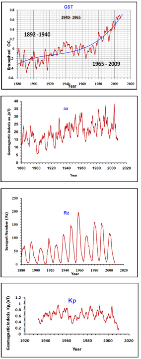Figure 1. The 12-month running averages of GST, aa, Rz, and Kp

It should be noted that global climate system has displayed irregular and progress changes (or increases) during the second half of the 20^th century to the beginning of the 21^st century, especially for the last four decades (1970-2009). Thus, the interesting to this subject is therefore continually increasing. The temperature variability showed a strong warming trend over the earlier period (+0.13 ºC/decade for 1892-1940 epochs) rather than for the past 40 years (0.2 ºC/decade for 1965-2009 epoch). The increase in GST throughout the second warming phase was faster and smoother than in the earlier years.

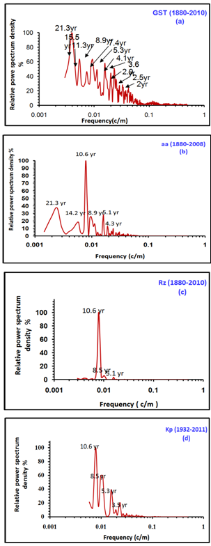Figure 2. The normalized power spectra density for the GST, the geomagnetic indices aa and Kp and the sunspot number Rz

The 2008 meteorological year was the warmest year over the record (+0.78 ºC), while the second and third warmest years were 2003 (+0.64 ºC) and 1998 (+0.58 ºC), respectively. Therefore, there has been a strong warming trend (0.56 ºC/decade) over the past yrs from 1996 to 2006. Temperatures have increased, and reflected a warming of approximately 1.2 ºC since 1892. On the other hand, the constant period maintained of high temperatures and it had a tendency (or behaviour) to slowly cooling. These results might have progressively played a dominant role in the global climate change during the last few years.

Plot b of Fig.1 displays the time series of 12-month averages for aa, Rz, and Kp. Plot (1c) illustrates that Rz has a cyclic variation with a minimum reaching the same level of the preceding cycles, while Plot (1b) displays the monthly aa running means, showing the increasing trend of aa with double peaks during the maxima solar activities. Some periodic structures are seen.

The power spectral density (PSD), describes how the power of a signal or time series is distributed with frequency. Here power can be the actual physical power, or more often, for convenience with abstract signal, can be defined as the squared value of the signal. This instantaneous power (the mean or expected value of which is the average power) is then given by:

The PSD is the Fourier Transform of the normalized autocorrelation function of lag, of the signal if the signal can be treated as a stationary random process.

The power of the signal in a given frequency band can be calculated by integrating over positive and negative frequencies,

The power spectral density of a signal exists if and only if the signal is a wide-sense stationary process. If the signal is not stationary, then the autocorrelation function must be a function of two variables, so no PSD exists, but similar techniques may be used to estimate a time-varying spectral density.

Relative power spectrum density =

For a comparison between GST and aa, we notice the following: during the period 1970-2008, the aa geomagnetic magnitude values have greatly increased than the previous years. The largest peak, over the considered period was in 2003, and the warmest year was 2008, of 5-yr apart. The second largest peak of geomagnetics aa was in 1992 corresponding to the third warmest peak (1998) in GST. El-Borie’s hypothesis displayed that the present changes in aa geomagnetics may reflect partially some future changes in the global surface temperatures[7] . The magnitudes of aa have greatly increased throughout the last four decades and the highest peak over the considered period was found in 2003 corresponding to the warm year was 2008. On the other hand, the second largest peak in aa spectrum occurred in 1992. For comparison, the separation-time between the second warmest year in 2003 and the greatest geomagnetic is about a few years, which may be indicated that the geomagnetic index aa is a considerable future factor on the magnitude of the global surface temperature with a lag time.

Fig (2) shows the power spectral density analysis of global surface temperature (GST), geomagnetic indices (aa), (Kp) and sunspot number (Rz). A series of power spectral density (PSD) have been performed for the 12-month running averages throughout the period (1880-2008). The results were smoothed using the Hanning window function and each spectrum is independently normalized to the largest peak in the complete spectrum. The power spectrum density is calculated for the wide range of frequencies (2.5x10^-3 - 0.5 c/m), which corresponding to a range from 33.3 year to 1 month.

Plots show that there are no significant peaks observed in the high-frequency region > 4x10^-2 c/m corresponding to the period from 1 month to less than 2 yr. A flat spectrum for the short-term fluctuations is observed. At the selected frequencies (>5 yr) the spectral density is high and it shows significant variations.

Significant peaks are observed (plot 2a) for the global surface temperatures at wavelengths of 21.3, 15.5, 11.3, 8.9, 7.4, 5.3, 4.1, 3.6 and 2.9-2 yr, while (plot 2b) of aa displayed peaks at wavelengths 21.3, 14.2, 10.6, 8.9, 5.1 and 4.3 yr. In addition, the spectra of Rz shed the significant peak at 10.6 yr. In (plot 2b), the aa spectrum reflected the same remarkable peak of 10.6 yr with high amplitude. Also in (plot 2d) of Kp displayed peaks at wave length 10.6, 8.5, 5.3, and 3.5 yr. We found similar fluctuations of 21.3, 10.6-11.6, 8.9, 5.1-5.3 between aa and GST. Also, we found similar peaks 21.3, 10.6, 8.5-8.9 between Rz & GST.

Table 1. displays the existed spectra period for each selected parameter Period Year Main period existence significant aa Kp Rz GST 3 – 4.5 4.3 3.5 ----- 3.6 , 4.1 5 - 7 5.1 5.3 ----- 5.3 8.5 - 8.9 8.9 8.5 ------ 8.9 10.6-11.3 10.6 10.6 10.6 11.3 14.2-15.5 14.2 ----- ----- 15.5 21.3 21.3 ------- ------- 21.3

Table 1 displays the existed spectra period for each selected parameter. The observed spectra of GST showed peak of 21.3 yr, which it is related to the solar magnetic cycle polarity reversals (Hale cycle). Another peak of 10.6 yr is seen with lower magnitude than that of 22-cycle obviously[28] . The 10.6 yr appear in spectra of aa, Kp and Rz with a little shift in GST spectrum. Additionally, GST spectrum contains minor peaks between 5-7yr which also displayed 5.3yr in Kp. The 5.3 yr is probably due to different paths of ion particle into the heliosphere for epochs of different solar magnetic cycle[29] . The 21.3 yr was observed in aa spectrum with large significant magnitude rather than Rz spectrum, so we can say that aa is more effective on global surface temperature than solar activity. Furthermore, the global surface temperature are strongly sensitive to the 21.3-yr, 10.6-yr, and 5.3-yr variations that observed in the considered geomagnetic and sunspot spectra.

4. Conclusions

The aim of this paper is relation in the longer time (1880-2011), between changer of global surface temperature (GST), and solar geomagnetic activist represented by sunspot number (Rz) and geomagnetic indices (aa , Kp ), and to what degree they are connected. Results of spectral analysis revealed strong 21.3 yr peak in GST than the 10.6 yr peak. It is related to the changes in the polarity of main solar magnetic field; this obtained result demonstrate that the interplanetary magnetic field (IMF) effect is more powered on GST than the solar activity cycle. Significant peak at 10.6 yr are appear in aa, Kp and Rz series which is the most established cycle of solar activity. We also found that 10.6 year peak in Rz series is larger than the same peak in aa series this indicate the geomagnetic activity predominate over the solar activity in GST.

The geomagnetics aa are more effective on global surface temperature than solar activity. Furthermore, the global surface temperature are strongly sensitive to the 21.3-yr, 10.6-yr, and 5.3-yr variations that observed in the considered geomagnetic and sunspot spectra. The present changes in aa geomagnetics may reflect partially some future changes in the global surface temperatures.