1. Introduction

The states in nature typically change in time. The importance in the investigation of these changes in complex systems helps to understand and describe such changes. A relatively new method based on non-linear data analysis has become popular to describe the changes of these systems. This method is called recurrence plot (Eckmann, 1987; Tanio, 2009).

Recurrence-based methods have a potential for representation of measurements from complex systems. However, it is necessary to determine the time intervals and state space subsets in which the stationary assumptions are hold (Yang et al., 2011).

This contribution makes the first approach in quantify and analyze the non-linear behavior of harmful airborne particles at various sites at London, England using recurrence features embedded in the raw datasets.

2. Background

2.1. Urban Airborne Pollution

In recent times, urban air pollution has been a growing problem especially for urban communities. Size, shape and chemical properties govern the lifetime of particles in the atmosphere and the site of deposition within the respiratorytract. Health effects differ upon the size of airborne particulates (Yin et al., 2010).

Air pollution has become a real concern, particularly in large urban locations (Kilabuko et al., 2007; Mirasgedis, 2008). Also, air pollution has been held responsible for various health disorders, especially respiratory complications resulting in an increase in the number of asthmatic cases and hospital admissions in some parts of the world and has been widely documented (Liu, 2011; Weinmayr et al., 2010; Arbex et al., 2010; Guo et al., 2010).

In this contribution, five airborne particles have been chosen mainly due to their impact on human health and data availability at the proposed sites. The datasets are separated according to month of the year and type of particle. There is one data for each hour, for each particle for all four London’s sites, making it difficult to extract information from datasets. The airborne particles analyzed in this paper are Sulphur dioxide (SO₂), Nitrogen Oxide (NO), Nitrogen Dioxide (NO₂), Carbon Monoxide and particulate matter (PM).

2.2. London’s Sites

London is the largest urban area and capital city of the United Kingdom. Greater London covered an area of 1,579 square kilometers. A larger area, referred to as the London Metropolitan Region covered an area of 8,382. (Sumbler et al., 1996)

There are a number of monitoring sites that are available in London, England. For this work, only four sites were chosen due to the availability of the data for the five particles used in this research. These sites are: London Bexley, Bloomsbury, London Marylebone Road and London North Kensington.

London Bexley’s site is located about 13 meters above the ground in a suburban area around 200 meters from A206 Northend Rd. and 300mts from Thames Rd. London Bloomsbury site is located within a self-contained unit at the north-east corner of a central London gardens. All four sides of the gardens are surrounded by a busy 2 lane one-way road system, which is subject to frequent congestion. The nearest road lies at a distance of approximately 25 meters from the station. The manifold inlet is approximately 3 meters high. (Defra, 2009)

Furthermore, London Marylebone Road site is located in a self contained cabin on Marylebone Road opposite Madame Tussauds. The manifold inlet is located at a height of 3 meters from the ground. The nearest road, the A50 is approximately 1 meter from the station. Traffic flows of over 80,000 vehicles per day pass the site on six lanes. The road is frequently congested. Lastly, the site at London North Kensington is located within a self contained cabin in the grounds of Sion Manning School. The manifold inlet is approximately 3 meters from the ground. The nearest road is a quiet residential road approximately 10 meters from the station. The surrounding area is mainly residential (Defra, 2009).

2.3. Recurrence Plots

Recurrence Plot (RP) is a graphical tool introduced by Eckmann (1987) in order to extract qualitative characteristics of a time series. The recurrence of a state I at a different time j is pictured within a two-dimensional squared matrix with black and white dots, where the black dots represent a recurrence and both axes represent time (Zbilut et al., 1998; Aboofazeli, 2008).

Such RP can be mathematically expressed as:

(1)

where, N is the number of considered states xi; is a threshold distance, a norm and (.) the Heaviside function (Furman, 2006).

Since by definition, the RP has a black main diagonal line called line of identity (LOI). In this context, the Heaviside function (.) is a recurrence of a state that is sufficiently close to (states that fall into an m-dimensional neighborhood) (Bradley et al., 2002).

Using the time series of a single observable variable (particles, in this case), it is possible to reconstruct a phase space trajectory. Starting from the scalar time series a sequence of embedded vectors

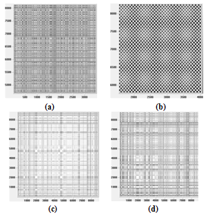
is generated (Palmieri et al., 2009). The set of all embedded vectors , constitutes a trajectory in where m is the embedding dimension and τ is the time delay. Each unknown point of the phase space at time I is reconstructed by the delayed vector in an m-dimensional space called the reconstructed phase space.

According to several authors, determining the embedding parameters should be the first step for nonlinear analysis (Marwan, 2002; Palmieri et al., 2009; Gao et al., 2000; Aparicio, 2008). As recurrence plots are highly sensitive to several of the features mentioned previously; a small change in one of these parameters can change the appearance of recurrence plots significantly (Rohde et al., 2008). Therefore, a search for the best dimension and time delay must be made first. In this appraisal, the best dimension value is calculated using the algorithm of false nearest neighbors (FNN) as shown on (Zou, 2010; Palmieri et al., 2009).

Also, when calculating an RP a norm must be chosen [Karakasidis et al 2009]. The most widely used norms are the L1, L2 (Euclidean norm) and L∞ (Zbilut, 2002).

For this contribution, the Euclidean norm was used. Figure 1 shows the recurrence plots of a random signal, a sine wave and two RPs chosen randomly for airborne particle concentration.

Figure 1. Recurrence Plots using (a) a random signal, (b) a sine wave, (c) particle concentration of carbon monoxide at London Bexley for 2010 and (d) particle concentration of sulphur dioxide over 2010 at Marylebone Road (daily mean) showing the Line of Identity (diagonal line).

Although it is possible to identify each plot from figure 1 (c and d), some experience is needed to interpret the RPs (Zbilut, 2007). For this reason, recurrence quantification analysis (RQA) offers a window to characterize RP structures.

The main idea of this project is to reconstruct the (unknown) system dynamics in the phase space by using time- delay embedding, and then computing the distances between all pairs of embedded vectors, generating a symmetric two-dimensional square matrix for each dataset as shown on figures 1c and 1d, applying RQA to each dataset.

2.4. Recurrence Quantification Analysis (RQA) for RPs

Zbilut (1998) and Webber (1994) have developed some of the methods used today for Quantitative Analysis of the recurrence plots. It has been shown that these measures are able to capture dynamical transitions in complex systems (Zuo et al., 2010). They define measures of complexity using certain characteristics of the recurrence plots (March et al., 2005; Marwan, 2007).

In general, the characteristics measured in a RP are: recurrence rate, determinism, ratio, entropy and trend.

2.4.1. Recurrence Rate

The recurrence rate is a measure of recurrences, or density of recurrence points in the RP. This rate gives the mean probability of recurrences in the system (Marwan, 2007; Strozzi et al., 2007). The recurrence rate is given by:

(2)

in the case of time series, and;

(3)

in the case of spatial data [Mocenni et al, 2011].

The recurrence rate represents the fraction of recurrent points with respect to the total number of possible recurrences. It is a density measure of the RP.

2.4.2. Determinism

Determinism is a measure for predictability of the system (Aparicio, 2008). The determinism could also be explained as the percentage of recurrent points forming line segments which parallel the Line of Identity (LOI). The determinism characteristic is given by (Gao et al., 2000):

(4)

Where P(l) denotes the probability of finding a diagonal line of length l in the RP. This measure quantifies the predictability of a system (Zou et al., 2010). The measure of determinism (DET) ranges from 0 to 1. Numbers near zero indicate randomness while those approaching one indicate the presence of a strong signal component (Furman et al., 2006; Ahlstrom, 2006).

The average diagonal line length L_mean is defined as:

(5)

This characterizes the average time that two segments of a trajectory stay in the vicinity of each other, and is related to the mean predictability time (Zou et al., 2010).

The choice of l_min can also be used in order to exclude short temporal scales that are not important. (Karakasidis, 2009)

2.4.3. Ratio

The Ratio variable is defined as the quotient of determinism (DET) divided by the recurrence (REC). It is useful to detect transitions between states: this ratio increases during transitions but settles down when a new quasi-steady state is achieved (Palmieri et al., 2009).

2.4.4. Entropy

The measure characteristic entropy refers to the Shannon entropy of the frequency distribution of the diagonal line lengths (Yulmetyev et al., 1999). According to several authors, the basic idea is that information (Shannon) entropy of the random processes is abundantly supplied with the qualitative and quantitative data on the object under research (Marwan, 2002; Yulmetyev et al., 1999; Strozzi et al., 2007; Karakasidis et al., 2009). The entropy of a system is given by:

(6)

2.4.5. Trend

The trend is a linear regression coefficient over the recurrence point density of the diagonals parallel to the LOI. The trend measurement is given by:

(7)

3. Experimental Results

Recurrence Quantification Analysis have been carried out for years 2005-2010 for all four sites mentioned in section 2.2 using the raw data (hourly) obtained from DEFRA (Defra, 2009) for each particle. The recurrence rate (REC), determinism (DET), Ratio, Entropy (ENT) and Trend have been modeled using Matlab® software. The results were analyzed separately and then put them together to present results altogether in form of boxplots. This analysis is complex due to the large quantity of the datasets.

There is much useful information that can be extracted from the recurrence plots using RQA. Figure 2 shows the recurrence rate for all particles.

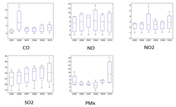Figure 2. Recurrence Rate for Particle Concentration, years 2005-2010.

In figure 2 is shown the recurrence Rate for all five particles (CO, NO, NO₂, SO₂ and PMx. In this figure, it is worth notice that the median recurrence rate for CO, NO NO₂ and PMx lies from 3 to 6, with the lowest recurrence rate being for nitrogen dioxide. However, Sulphur dioxide shows a much higher recurrence rate with an average of 29 increasing in some regions of London Bloomsbury to 44. This higher recurrence rate may be due to the low variances in values of the datasets for all years, making it easier for RQA to determine recurrence.

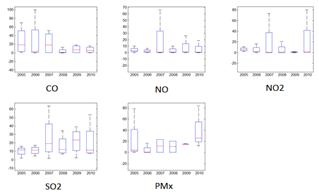Figure 3. Determinism for Particle Concentration, years 2005-2010.

Furthermore, the determinism for SO₂ is also higher than for other particles, having a median of 18 as shown on figure 3. Although it seems lower due to the scaling of the boxplots, the median shows otherwise, the spread in the 25th to 75th percentiles and the length of the whiskers may be due to exceptionally high determinism for that site in particular or an outlier and not necessarily represent a higher determinism altogether.

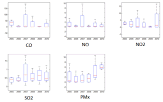Figure 4. Ratio for Particle Concentration, years 2005-2010.

Furthermore, it is worth notice for entropy that the frequency distribution of the data is slightly higher for particle concentration CO than for the other particles. The other particles seem to have steady entropy whose median oscillates between 3 to 5 with a few exceptions (i.e. PMx2006, 2009). This is shown on figure 5.

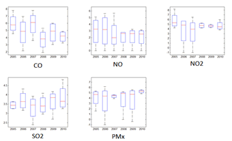Figure 5. Entropy for Particle Concentration, years 2005-2010.

The last measure was the trend. Since the trend represents the measure of the positioning of recurrent points away from the central diagonal, that is the paling of the RP towards its edges (Palmieri et al., 2009). A ‘‘flat” diagram indicates stationarity, whereas drift in the signal will result in the overall increase or reduction of distances as the signal is moved away from the main diagonal. In this respect, it could be noticed that most of the particles have a median between -0.5 to 0.5. There are a few exceptions such as SO₂ for 2010 and PMx for 2010. The reason could not be ascertain for sure, hence further investigation is recommended. This is shown on figure 6.

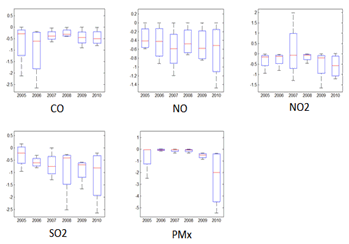Figure 6. Trend for Particle Concentration, years 2005-2010.

4. Conclusions and Future Work

Numerous experiments have been carried out with different particles and through different years. Using Recurrence Quantification Analysis it could be shown that information could be extracted from large datasets of dissimilar airborne particles during a considering time lap (six years, in this case). Trends could be identified using these tools and preliminary conclusions suggest that important information such as density distribution, drifts, among others could be drawn.

For future work, it could be useful to use a combination o RQA with prediction algorithms such as Support Vector Machines to carry out prognosis of the airborne particle data. Another useful approach that could be carried out is the use of cross recurrence plot (CRP), making a comparison between two recurrence plots to determine trends.

ACKNOWLEDGEMENTS

The authors would like to thank Alan Charton from The Air Quality Archive hosted by AEA Energy & Environment, on behalf of the UK Department for Environment, Food & Rural Affairs and the Devolved Administrations (DEFRA). Also, the authors would like to acknowledge the financial support of the Mexican government via PROMEP funding.