-
Paper Information
- Paper Submission
-
Journal Information
- About This Journal
- Editorial Board
- Current Issue
- Archive
- Author Guidelines
- Contact Us
American Journal of Condensed Matter Physics
p-ISSN: 2163-1115 e-ISSN: 2163-1123
2017; 7(2): 50-56
doi:10.5923/j.ajcmp.20170702.03

Contribution to the Understanding of III-V Based Nanohole Filling
 Abstract
 Reference
 Full-Text PDF
 Full-text HTML
Antal Ürmös, Zoltán Farkas, Ákos Nemcsics
Institute of Microelectronics and Technology, Óbuda University, Budapest, Hungary
Correspondence to: Antal Ürmös, Institute of Microelectronics and Technology, Óbuda University, Budapest, Hungary.
| Email: |  |
Copyright © 2017 Scientific & Academic Publishing. All Rights Reserved.
This work is licensed under the Creative Commons Attribution International License (CC BY).
http://creativecommons.org/licenses/by/4.0/

A model of filling dynamics of nanoholes will be detailed in this paper. The filling material will be modelled as a viscous liquid. The structure of this paper is as follows. The forming of nanoholes will be briefly described and the filling of these nanoholes will be detailed with and without surface diffusion. The modelling algorithm will be shown for InAs / InGaAs substrate. The description of the modelling algorithm, one possible microscopic interpretation of the viscosity will studied as well. In addition, the number of layers and the equilibrium height relation will be investigated at different temperatures. Furthermore both the viscosity and equilibrium height will be investigated as the function of the temperature. Out investigations will be carried out at macroscopical and microscopical levels as well.
Keywords: Nanohole-filling, Droplet epitaxy, GaAs, Modelling, Simulation
Cite this paper: Antal Ürmös, Zoltán Farkas, Ákos Nemcsics, Contribution to the Understanding of III-V Based Nanohole Filling, American Journal of Condensed Matter Physics, Vol. 7 No. 2, 2017, pp. 50-56. doi: 10.5923/j.ajcmp.20170702.03.
Article Outline
1. Introduction
- The number of utilization of nanostructures grows permanently. Examples for this the production process of LEDs [1], lasers [2] and GaAs based solar cells [3]. The construction of these GaAs based devices depends to a large extent on fabricating both semiconductor crystal layers and nanostructures. The fabrication process is carried out primarily with molecular beam epitaxy (hereinafter MBE) [4, 5]. Different structures are produced by different methods. A widely used method for the growth of quantum dots is the Stransky-Krastanov method. A relatively new method is the droplet epitaxy which is based on the Volmer Weber method. The principle of droplet epitaxy was invented by Koguchi et al. at the beginning of 1990’s. The first step of this process is a deposition of a III main group (eg. In or Ga) droplet onto the substrate (eg. GaAs or AlGaAs). During the second step, the droplets crystallizes and nanostructures are formed. The type of nanostructure is determined as a function of both the pressure of gas phase of V main group element (eg. arsenic) in the environment of the droplet and the temperature of the substrate. This method is useful to produce quantum rings [10], nanoholes [11] and other nanostructures, in addition to quantum dots. Inverse technology quantum dots can be also produced by filling nano holes [12, 13]. A good review on this subject is [14].Nano holes are produced by local thermal etching on AlGaAs substrate at temperature of T=550-640°C. It is possible to carry out partial or complete burying in case of nano holes. Elevations of size of some nanometers can be observed above the buried quantum dots [14]. Vertically stacked quantum dot molecule can be produced by sequential filling. This structure contains two closely positioned quantum dots. That is the simplest system of interacting nanostructures. Vertically stacked quantum dots consist of two twice buried quantum dots of ultra-low density. In case of GaAs/InAs substrate the dots are separated by a GaAs barrier of a well-defined width. In case of AlGaAs/GaAs substrate, the separating barrier is of AlGaAs. According to the literature there are experimental results of GaAs inverted quantum dots produced on AlGaAs substrate and InAs and InGaAs inverted quantum dots on GaAs substrate. In this paper the model of filling a nanohole created with In/Ga droplet on GaAs substrate is presented. The filler material is InAs/InGaAs.
2. Details of the Simulation Algorithm
- Our model takes into consideration only the movement of metal component because the location of transformation into semiconductor state (crystallization) is not influenced by the non-metallic component according to the experiments [11]. The initial parameters are illustrated on Figure 3. Dring is the width of the ring (the difference between the outer circle radius and inner circle radius). The Dhole is the diameter of the hole, L is the height of the ring above the substrate, H is the height of the ring above the bottom of the hole. Parameter
 is the half angle of the orifice of the hole. This angle is 55°. The parameters are explained on Figure 1.In each step, 2 monolayers of Indium were deposited. The layers were stacked onto each other. The atoms migrate on the surface during the growth interrupt. For more information about the filling process, please see the ref. [11]. The In atoms deposited from evaporated gas phase.
 | Figure 1. The structure of the investigated nano hole, where (a.) is the area surrounding the nanohole, (b.) ring, around the nanohole and (c.) is the nanohole. The “itc” index is the abbreviation of the inner truncated cone |
 | (1) |
 | (2) |
3. The Inclusion of Atomic Movement
- If one wishes to present a realistic model the atoms move on the surface of the substrate at (n *k *T > Ebonding) temperature. This movement can be modelled in several ways, eg. a Kinetic Monte-Carlo method [17, 18]. In this paper the temperature dependent dynamic viscosity of liquid Indium will be taken into consideration instead. In a macroscopic context dynamic viscosity is a proportional factor, which depends on the properties of the liquid. This factor shows the relation between the shear stress and the deformation velocity, which can be calculated by the τ=μ*dγ/dt formula. In this equation, τ is the shear stress, μ is the dynamical viscosity and the dγ/dt is the deformation velocity.This viscosity can be calculated in different ways for liquid metals [19-23]. In this paper the Arrhenius-Andrande formula will be used [23]:
 | (3) |
 is the bulk activiation energy (in case of Indium 6650 J/mol), and
  is universal gas constant (8,3144 J/(K*mol)).In nanoscopic approach the probability of occurring of an event must be determined at atomic level dynamic [18, 17]:
 | (4) |
 | (5) |
 | (6) |
 | (7) |
 is the filled up thickness in step, and
  is the sum of volumes deposited from 1-st step to the i-th step. Variable α is the half angle of the orifice of the hole (55°). As a consequence, the value π*tg255 = 6.4.
 | Figure 2. Illustration of volumes deposited onto different parts of the nanohole after depositing two layers. The first deposited layer appears in dark blue, the second deposited layer is light blue. The thickness of the layer on the ring and aside the ring is δ. There is no diffusion in case (A), there is diffusion in the case (B). The arrows illustrate that proportion (1-η) * λhole (where λhole = rhole / rtc) of the volume on the ring gets into the orifice. The λhole is the radius proportional factor of the nanohole, rhole is the radius of the nanohole and rtc is the radius of the entire truncated cone. The (1-η)*(1- λhole) part gets to the environ of the nanohole. For detailed description, see the next chapter |
4. Evaluation and Discussion
- The object of our interest was to examine how the nanohole gets filled with deposited Indium as a function of substrate temperature before the Indium crystallizes. During the filling process the height of the ring that surrounds the nanohole grows as well. In other words, we looked for the phase of In deposition at which the height of material covering the nanohole and the height of the ring are equal. The two heights are considered equal if the respective difference is between zero and one. The average of the two heights is the equilibrium height. During the simulation we sought the temperature at which the height difference of a given deposition layer is minimal.On Figure 3 the filling process of the nanohole is shown. If the temperature dependence of the viscosity is considered negligible then the height equivalence appears at the 21st layer. The Reader should take into consideration that each deposited layer implies that two monolayers are deposited.
 | Figure 3. The filling process of the nanohole, in case of 1 (A), 7 (B) layers |
 | Figure 4. Layer number and equilibrium height diagrams at different temperatures |
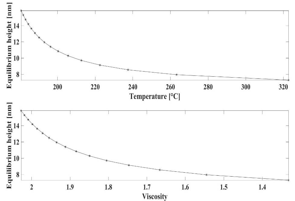 | Figure 5. The temperature-equilibrium height (top), and the viscosity-equilibrium height (bottom) diagrams |
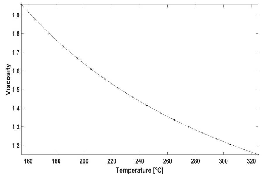 | Figure 6. The macroscopic temperature-viscosity diagram of Indium |
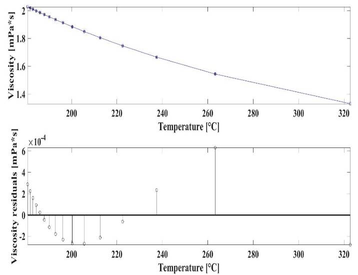 | Figure 7. The nanoscopic temperature-viscosity diagram. In this figure, a power-law function is fitted to the point series. In the top part the fitted power-law function and in the bottom part the absolute error of the fitting is shown |
 are 1.398*1014, -0.06772, 22.77, -0.001933 respectively. Again, the upper diagram is the function fitted to dot sequences, the lower diagram is the absolute error of the fitting at each point. The maximal value of the fitting error is 0.1548 (the relative error is 1.94%), that can be found at 263.35°C (536.5 °K).
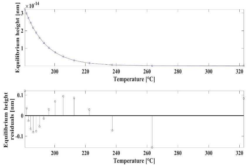 | Figure 8. The nanoscopic temperature-viscosity diagram. In this figure, an exponential sum function is fitted to the point series. In the top part the fitted exponential sum function and in the bottom part the absolute error of the fitting is shown |
5. Conclusions
- A possible model of the filling of nanoholes was discussed in this paper. The filler material was modelled as a viscous liquid. During the simulation the behaviour of the In was investigated in heated substrate during the evaporation. First, the case was investigated, when there is not surface diffusion, so there is no atomic displacement on the surface. After this, the atomic displacement was considered, so that the atomic ensemble was regarded as the viscous liquid, the movement of which corresponds to the surface diffusion. Next to the description of the modelling algorithm, one possible microscopical interpretation of the viscosity was studied as well. In addition, the layer number and the equilibrium height relation was investigated at different temperatures. Furthermore, the viscosity was investigated as a function of the temperature and the equilibrium height as a function of the temperature as well. Our research covered both the macroscopic and microscopic level. The equilibriums height depends on the temperature.