Nelson O. Nenuwe1, John O. A. Idiodi2
1Department of Physics, Federal University of Petroleum Resources, Effurun, Nigeria
2Department of Physics, University of Benin, Benin City, Nigeria
Correspondence to: Nelson O. Nenuwe, Department of Physics, Federal University of Petroleum Resources, Effurun, Nigeria.
| Email: |  |
Copyright © 2015 Scientific & Academic Publishing. All Rights Reserved.
Abstract
Contrary to the usual Fermi liquids, where the exponent of the momentum distribution at k=kF is fixed to an integer, for the Tomonaga-Luttinger (TL) liquids the anomalous exponent of the momentum distribution changes continuously, resulting in a power-law singularity of the momentum distribution function. It has been said that this power-law singularity appears at kF and 3kF for the Hubbard model as well as at kF for the t-J model. Using the conformal field theory (CFT) technique, we present an exact calculation of the anomalous exponent of the t-J model at kF, 3kF, 5kF and 7kF and compare it with the results for the Hubbard model.
Keywords:
Tomonaga-Luttinger liquid, Momentum distribution, Power-law singularity
Cite this paper: Nelson O. Nenuwe, John O. A. Idiodi, Tomonaga-Luttinger Anomalous Exponents of kF, 3kF, 5kF and 7kF Momentum Distribution in the t-J Model, American Journal of Condensed Matter Physics, Vol. 5 No. 1, 2015, pp. 19-39. doi: 10.5923/j.ajcmp.20150501.03.
1. Introduction
Since the original work on high-Tc superconductivity in the 80’s by Bednorz and Muller [1], the interest in studying highly correlated electron systems in low-dimension has greatly increased. It is usually believed that one-dimensional (1D) systems are the simplest to discuss electron correlation problem [2]. Haldane [3] introduced the theory of TL liquid that is valid in understanding the low-energy behaviour of a large class of 1D correlated models. The role of Fermi liquid (FL) in three dimensions is replaced by TL liquid in 1D. The remarkable feature of TL liquids is the absence of a finite jump discontinuity in the momentum distribution function  at the Fermi momentum,
  and the presence of power-law singularity near the Fermi point, which corresponds to collective motion of Fermions instead of quasi-particle excitations. The efforts to find appropriate model to clarify the non-Fermi liquid behaviour of low-dimensional highly correlated systems, led to series of numerical and analytical investigations. Significant progress was made by Parola and Sorella [4] and Ogata and Shiba [5] for the Hubbard model. This also motivated Kawakami and Yang [6] to calculate the correlation exponents in 1D correlated systems and to clarify their TL liquid nature. In fact, Kawakami and Yang calculated the long-distant behaviour of correlation functions at
  in the t-J model at
  . The critical exponents (
 at
at  and
and  at
at  ) obtained numerically by these authors is in agreement with analytical predictions for the Hubbard model. However, it is hard to determine numerically the exact nature of the singularity at
  . Since the anomalous exponents around
  and
and  has not been calculated yet for the t-J model, our aim in this paper is to follow the work of Kawakami and Yang [6], and extend their work by calculating the anomalous exponents of the momentum distribution function
  around the Fermi points
  using the CFT technique.
2. Finite-Size Scaling in Conformal Field Theory
The conformal dimensions are obtained from the Hamiltonian [7] of 1D t-J model defined by 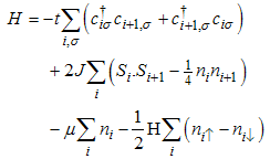 | (1) |
Where  is the spin-
 electron creation, annihilation operators at the ith site,
 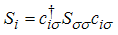 is the spin
  matrix S,
 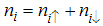 is the number operator with
  , and
, and  and H are the chemical potential and the external magnetic field, respectively. Equation (1) has been solved exactly by Kawakami and Yang to obtain the Bethe Ansatz equations
 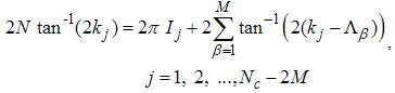 | (2) |
and | (3) |
with  and
and as spin rapidities
 | (4) |
The state corresponding to the solution of the Bethe Ansatz equations has energy and momentum given by | (5) |
 | (6) |
Where the conformal dimensions are given by  | (7) |
 | (8) |
The non-negative integers  , where
  (holon) and
  (spinon) describes particle-hole excitations, with
  being the number of occupancies that a particle at the right (left) Fermi level jumps to,
  represents the change in the number of electrons (down-spin) with respect to the ground state,
  represents the number of particles which transfer from one Fermi level of the holon to the other and
  represents the number of particles which transfer from one Fermi level of the spinon to the other, and both
  and
and  takes integer or half-odd integer values. Lastly, Z is the dressed charge matrix defined by
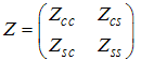 | (9) |
The elements of the dressed charge matrix are given by the coupled integral equations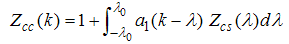 | (10) |
 | (11) |
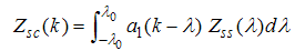 | (12) |
 | (13) |
The kernels are defined by | (14) |
Usually, the CFT expression for two-point correlation function of the scaling fields  with conformal dimensions
  for the t-J model takes the form
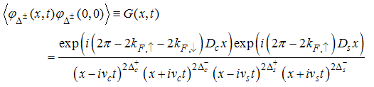 | (15) |
Where  and
and  are the Fermi momentum for electrons with spin up and down, respectively.
  and
and  are the Fermi velocities of charge and spin density waves and
  are constants.
3. Correlation Function
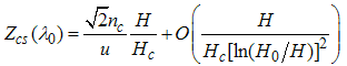
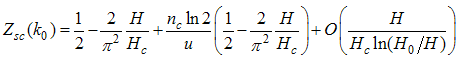
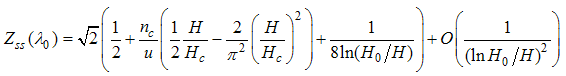
For small magnetic field  , we solve the dressed charge matrix equations (10) to (13) by Wiener-Hopf technique [7, 8] and obtain (see Appendix A)
 | (16) |
 | (17) |
 | (18) |
 | (19) |
Using the dressed charge matrix elements Eqns. (16) to (19) on the conformal dimension Eqns. (7) and (8), we obtain [see (A72) and (A73)] 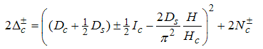 | (20) |
 | (21) |
Therefore, the long-distance behaviour of the electron field correlation function with up-spin is obtained from the set of quantum numbers  ,
,  ,
,  ,
,  ,
,  and
and  . For
. For  , the corresponding conformal dimensions are
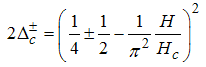 | (22) |
 | (23) |
 | (24) |
 | (25) |
Here, we have neglected contributions from  and terms of order
  .Using Eqns. (23) and (25) on (15), we obtain
 | (26) |
The critical exponent is given by  | (27) |
This implies that | (28) |
and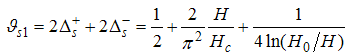 | (29) |
Next, for 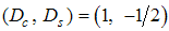 , we obtain the conformal dimensions as
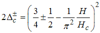 | (30) |
 | (31) |
 | (32) |
 | (33) |
Using Eqns. (33) and (31) on (15), we obtain | (34) |
Where the critical exponents are given by  | (35) |
 | (36) |
Also, the conformal dimensions for  , are
, are | (37) |
 | (38) |
 | (39) |
 | (40) |
Using Eqns. (40) and (38) on (15), we obtain | (41) |
 | (42) |
 | (43) |
Finally, the conformal dimensions for  are
are | (44) |
 | (45) |
 | (46) |
 | (47) |
Using Eqns. (47) and (45) on (15), we obtain | (48) |
The critical exponents are given by  | (49) |
 | (50) |
Combining Eqns. (26), (34), (41) and (48), we obtain the asymptotic form of the electron field correlator with up-spin as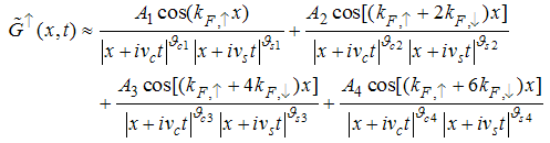 | (51) |
From Eqn. (51) it is clear that in the strong-coupling limit, the  singularity manifests itself as
  ,
,  manifest as
  and
and  as
as  . Therefore, the asymptotic form of the equal-time correlator of the electron field (with
  ) is given by
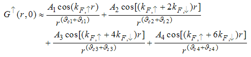 | (52) |
3.1. Correlation Function in Momentum Space
It is well known that the asymptotics of the two-point correlation function determines the singularities of the spectral functions [9] near  . The electron field correlation function in momentum space is obtained by Fourier transforming the asymptotic form obtained above. In fact, the result Eqn. (52) has singularities near the Fermi point
 and
and  respectively. Therefore, at the Fermi point
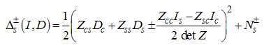
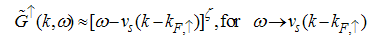
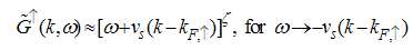
  , the momentum distribution takes the form (see Appendix B)
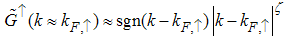 | (53) |
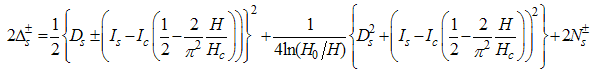
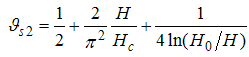
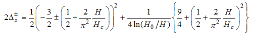
Where the anomalous exponent 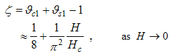 | (54) |
and  | (55) |
Here and in what follows, we neglect the logarithmic field dependence of the anomalous exponent. Therefore, the nature of singularities for the contributions with Fermi wave number  are obtained as
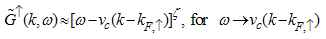 | (56) |
with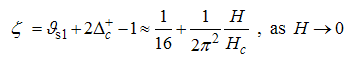 | (57) |
 | (58) |
with  | (59) |
 | (60) |
with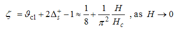 | (61) |
 | (62) |
with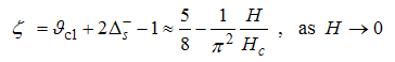 | (63) |
Eqn. (53) represents the momentum distribution function around the Fermi point  for the electron field correlation function. It exhibits a characteristic power-law singularity of the TL liquid, with exponent Eqn. (54). This anomalous exponent
  , for
, for  grows monotonically with increasing magnetic field. i.e.
  as
as  and
and  as
as  , hence the momentum distribution function in the presence of magnetic field exhibits a rapid change around
  as shown in figure 1.
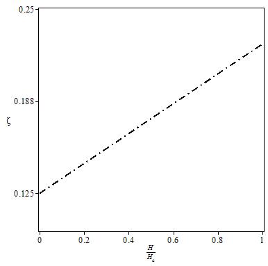 | Figure 1. The anomalous exponent  for the momentum distribution around for the momentum distribution around  as a function of as a function of  in the t-J model in the t-J model |
Next, at  , the momentum distribution is obtained as
  | (64) |
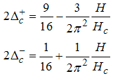
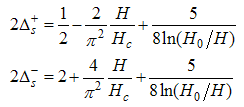
The anomalous exponent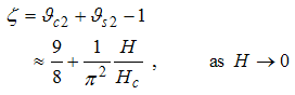 | (65) |
and | (66) |
The nature of singularities for 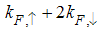 are obtained as
 | (67) |
with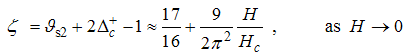 | (68) |
 | (69) |
with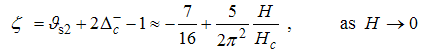 | (70) |
 | (71) |
with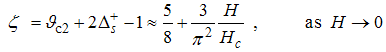 | (72) |
 | (73) |
with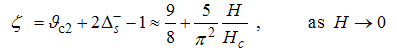 | (74) |
Also, Eqn. (64) represents the momentum distribution around the Fermi wave number  for the electron field correlator. It exhibits a characteristic power-law singularity of the TL liquid with exponent Eqn. (65). This anomalous exponent
  , grows monotonically from
  to
to  as the magnetic field goes from 0 to 1, and hence the momentum distribution function in the presence of magnetic field exhibits a rapid change around
  as shown in figure 2.
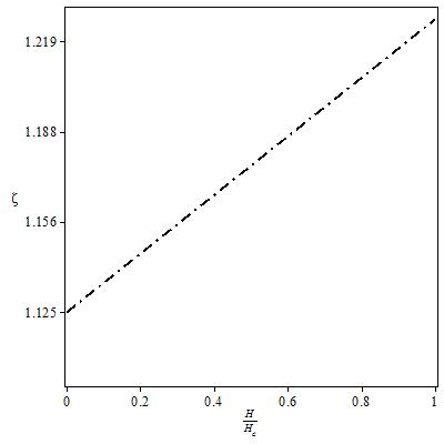 | Figure 2. The anomalous exponent  for the momentum distribution around for the momentum distribution around  as a function of in the t-J model as a function of in the t-J model |
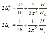
At  , the momentum distribution is obtained as
  | (75) |
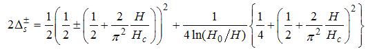
Where the anomalous exponent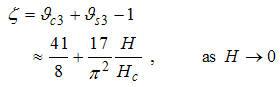 | (76) |
and | (77) |
The nature of singularities for  are
are | (78) |
with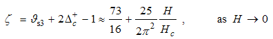 | (79) |
 | (80) |
with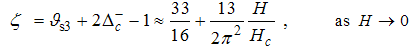 | (81) |
 | (82) |
with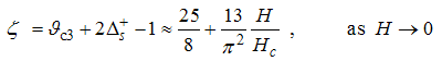 | (83) |
 | (84) |
with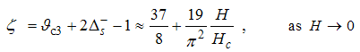 | (85) |
Eqn. (75) represents the momentum distribution function around the Fermi point  . It exhibits a characteristic power-law singularity of the TL liquid with exponent Eqn. (76). The anomalous exponent
  , grows monotonically from 5.125 to 6.847 as the magnetic field goes from 0 to 1, and hence the momentum distribution function in the presence of magnetic field exhibits a rapid change around
  as shown in figure 3.
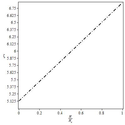 | Figure 3. The anomalous exponent  for the momentum distribution around for the momentum distribution around  as a function of as a function of  in the t-J model in the t-J model |
Finally, at  , the momentum distribution is obtained as
  | (86) |
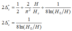
The anomalous exponent 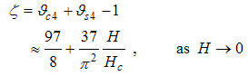 | (87) |
and | (88) |
The nature of singularities for  are
are | (89) |
 | (90) |
with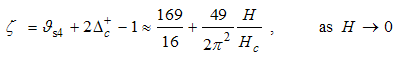 | (91) |
 | (92) |
with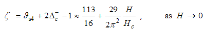 | (93) |
 | (94) |
with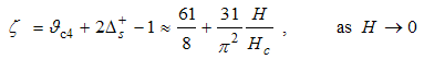 | (95) |
 | (96) |
with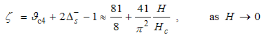 | (97) |
The momentum distribution Eqn. (86) around the Fermi point  also exhibits a power-law singularity of the TL liquid with exponent Eqn. (87). This anomalous exponent
  , grows monotonically from
  to
to  as the magnetic field goes from 0 to 1, and hence the momentum distribution function in the presence of magnetic field exhibits a rapid change around
  as shown in figure 4.
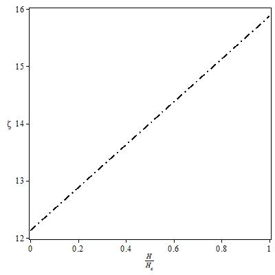 | Figure 4. The anomalous exponent  for the momentum distribution around for the momentum distribution around  as a function of as a function of  in the t-J model in the t-J model |
4. Discussion
In conclusion, the result Eqn. (52) has singularities near the Fermi points  and
and  respectively. The
  part arises from the excitation of
  , the
, the  part from
  , the
, the  part from
 and
and  from
from  . This implies that the
  part is dominated by spinon excitation alone. On the other hand both the holon and spinon excitations are responsible for
  and
and  oscillation parts respectively. We observed that the anomalous exponent,
  grows monotonically with increasing magnetic field. However, from Eqns. (54), (65), (76) and (87), at vanishing magnetic field the exponent,
  goes to
  for
for  ,
,  for
for  , 5.125 for
  and 12.125 for
  respectively. The values
  and
and  for
for  and
and  is in agreement with the evaluation for the Hubbard model by Ogata and others [5, 10, 11]. However, our exponents for the momentum distribution function at
  and
and  disagrees with the values of Shaojin and Lu [12] for the Hubbard model they obtained as
  and 1, respectively. Finally, the exponent for the momentum distribution function around
  is quite new. It indicates the presence of singularity and shows characteristic TL liquid property at this Fermi point.
Appendix
A. Wiener-Hopf technique for dressed charge matrixSome useful relations are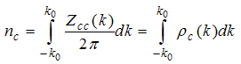 | (A1) |
and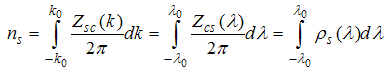 | (A2) |
Where,  is the density of down-spin electrons,
  is density of electrons,
  is the charge distribution function with holon momentum
  and
and  is down-spin distribution function with spinon rapidity
  . For small magnetic field
  , we solve the dressed charge matrix Eqns. (10) to (13) by Wiener-Hopf technique for only terms up to order
  in the strong coupling limit. With Eqn. (A2), we write Eqn. (13) as
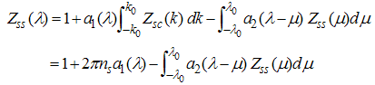 | (A3) |
Fourier transforming (A3), we obtain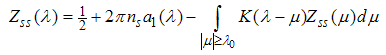 | (A4) |
Where the kernels are given by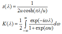 | (A5) |
We solve Eqn. (A4) by introducing the function | (A6) |
and expanding it as | (A7) |
Where  are defined as the solutions of the Wiener-Hopf equations
  | (A8) |
 | (A9) |
The driving terms  and the solutions
  becomes smaller as
  as increases because
  is large. Our procedure follows Fabian et al. [9]. Assuming the function
  and
and  are known. We define
 | (A10) |
Where the functions  are analytic on the upper and lower planes respectively, with
 | (A11) |
Also we assume | (A12) |
In terms of these functions we express the Fourier transform of Eqn. (A9) as | (A13) |
Where  is the Fourier transform of
  . Now we split (A9) into the sum of two parts that are analytical and non-zero in the upper and lower half planes. To obtain this we use the factorization
 | (A14) |
 | (A15) |
Where  are analytic and non-zero in the upper and lower half planes respectively and are normalized as
 | (A16) |
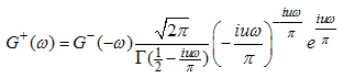
Useful special function of  are
are | (A17) |
Using (A13) and (A14), we obtain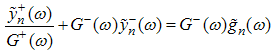 | (A18) |
Decompose the right hand side of (A18) into the sum of two functions | (A19) |
This implies that | (A20) |
To obtain the solution of (A8) for  , we set the driving term to be
 | (A21) |
We decompose the first term by using | (A22) |
The second term of (A21) is meromorphic function of  with simple poles located at
 | (A23) |
Note, there is no pole at  . The decomposition of the factor
  gives
gives | (A24) |
 | (A25) |
Using (A25) we can express the function  , for any function
  that is analytic and bounded in the lower half-plane as the sum of two functions
  analytic in the upper/lower half-plane
 | (A26) |
 | (A27) |
Applying the formula (A27) to (A21) and (A19), we obtain | (A28) |
 | (A29) |
Now, | (A30) |
Therefore, | (A31) |
 | (A32) |
For 
 | (A33) |
The functions  are obtained by using (A20)
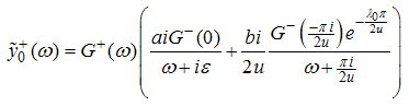 | (A34) |
From (A9) for  , by setting
 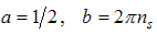 in (A34), we obtain
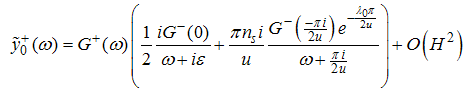 | (A35) |
By definition  | (A36) |
 | (A37) |
Where,  is magnetic field,
  is critical field,
  strong coupling,
  magnetic field at zero temperature and
  corresponds to Fermi points.Combining the result (A35) with (A36), we obtain the first the first order contribution to
  as follows
 | (A38) |
As  , we use Eqns. (A16) and (A17) on (A38) to obtain
 | (A39) |
Simplifying further, we obtain | (A40) |
Using (A37), we obtain | (A41) |
Next, the second order contribution to  is obtained by taking the Fourier transform of (A9) for
  .
. | (A42) |
From (A14) | (A43) |
 | (A44) |
From Eqn. (A19), | (A45) |
We have decomposed  into
into  which is analytic in the upper and lower half-planes.
  is given by
 | (A46) |
Where  is a small positive constant.
  has a branch cut along the negative imaginary axis and by deforming the contour of integration we rewrite (A44) as
 | (A47) |
From (A15), as 
 | (A48) |
 | (A49) |
Since, 
 | (A50) |
For  the integrand rapidly decrease because
  , and hence the integral is approximated by expanding the terms other than
  around
  . Therefore, we obtain
  | (A51) |
From (A20), we obtain | (A52) |
Using  | (A53) |
we obtain | (A54) |
From (A37) | (A55) |
Therefore, with (A39) and (A52), we obtain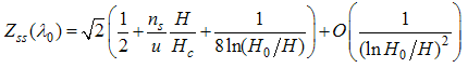 | (A56) |
Now to evaluate the dressed charge matrix element  , we take the Fourier transform of Eqn. (12) and (A4) and obtain
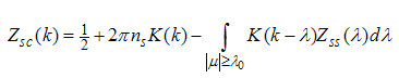 | (A57) |
Applying the same process in the determination of Eqn. (61), we obtain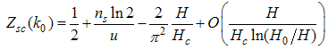 | (A58) |
Similarly, with the same process, we obtain the other two elements of the dressed charge matrix as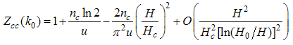 | (A59) |
and 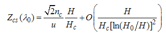 | (A60) |
From Eqn. (A2) together with the property that  for
for  and
and  , the down-spin density
  is obtained as
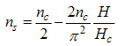 | (A61) |
Using Eqn. (A58) on (A53) to (A56), we obtain the dressed charge matrix equations as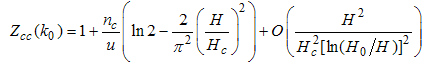 | (A62) |
 | (A63) |
 | (A64) |
 | (A65) |
At half-filling  , and by neglecting corrections to order
  , the elements of the dressed charge become
 | (A66) |
 | (A67) |
 | (A68) |
 | (A69) |
Derivation of conformal dimensions in terms of small magnetic fieldNote that,  | (A70) |
Using (A66) to (A69) on (A70) gives | (A71) |
Now, with Eqns. (A66) to (A69) on Eqns. (7) and (8), we obtain the magnetic field dependence of the conformal dimensions as | (A72) |
 | (A73) |
B. Correlation function in momentum spaceThe long-distance behaviour of the two point correlation function usually determines the singularities of spectral functions near 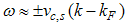 and the Fourier transform
  produces
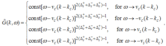 | (B1) |
and the Fourier transform of equal-time correlator is given by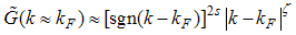 | (B2) |
Where the anomalous exponent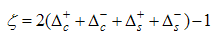 | (B3) |
and the conformal spin is | (B4) |
References
| [1] | Bednorz, J.B. and Muller, M.A. (1986). Possible high-Tc superconductivity in Ba-La-Cu-O system. Feitscchrift fur Physik B 64 (2), 189-193. |
| [2] | Anderson, P.W. (1989). Problem and Issues in the RVB theory of high-Tc superconductivity. Phys. Rep. 184, 195-206. |
| [3] | Haldane, F.D.M. (1981). Luttinger liquid theory of the one-dimensional quantum fluids. I. Properties of Luttinger model and their extension to the general 1D interacting spinless Fermi gas. Journal of Physics C: Solid State Physics, 14 (19), 2585. |
| [4] | Parola, A. and Sorella, S. (1990). Asymptotic spin-spin correlations of the  , one-dimensional Hubbard model. Phys. Rev. Lett. 64 (15), 1831-1834. , one-dimensional Hubbard model. Phys. Rev. Lett. 64 (15), 1831-1834. |
| [5] | Ogata, M. and Shiba, H. (1990). Bethe-Ansatz wave function, momentum distribution, and spin correlation in the one-dimensional strongly correlated Hubbard model. Phys. Rev. B 41 (4), 2326-2338. |
| [6] | Kawakami, N. and Yang, S-K. (1991). Luttinger liquid properties of highly correlated electron systems in one dimension. J. Phys. Condens. Matter 3, 5983-6008. |
| [7] | Anderson P.W. (1987). The Resonating Valence Bond State in La2CuO4 and Superconductivity, Science Vol. 235 No. 4793, 1196-1198. |
| [8] | Yang, C.N. and Yang, C.P. (1966). One-dimensional chain of anisotropic spin-spin interactions. II. Properties of the ground-state energy per lattice site for an infinite system. Phys. Rev. 150, 327-339. |
| [9] | Fabian, H. L. E., Frahm, H., Frank, G. O. H., Andreas, K. and Korepin V. E. (2005), The One-Dimensional Hubbard Model. Cambridge University Press, New York, 1-674. |
| [10] | Ogata, M., Tadao, S, and Shiba, H. (1991), Magnetic-Field Effect on the Correlation Functions in the One-Dimensional Strongly Correlated Hubbard Model, Phys. Rev. B 43 (10), 8401-8410. |
| [11] | Shiba, H. and Ogata, M. (1992), Properties of One-Dimensional Strongly Correlated Electrons, Prog. Theor. Phys. Suppl. 108, 265-286. |
| [12] | Shaojin, Q. and Lu, Y. (1996). Momentum distribution critical exponents for the one-dimensional large-U Hubbard model in the thermodynamic limit. Phys. Rev. B 54 (3), 1447-1450. |
 Abstract
 Reference
 Full-Text PDF
 Full-text HTML