1. Introduction

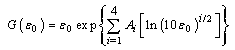
Positron-transport calculations are usually performed using either analytical theory or Monte Carlo simulation. Both methods require an accurate knowledge of the cross section for elastic scattering of electrons as function of the projectile kinetic energy E. Thus, the screened cross-section obtained via the first order Born approximation is extensively used in the literature. To model elastic scattering, Rouabah et al suggested a simplified expression of the positron transport cross-section (TCS), which depends only on the atomic number and based on Jablonski model[2] and their calculation has been done for the energy range 1-4 keV. Moreover, they said that their study gathered information which could be useful for the evaluation of parameters required for the quantitative low-energy positron annihilation spectroscopy (QLEPAS).

After a careful analysis of Ref.[1] we note that there is a problem in the expression of positron TCS.

In our recent paper[3], we have shown a short overview on some weak points of Rouabah et al paper[1]. So, the present work gives more detail on the majority of other Rouabah et al weak points especially the drastic deviation of their results. Therefore, the obtained results should be reviewed and revised as follows:

2. The Theoretical Background of the Commented Paper

2.1. The Correct Expression of the Jablonski Transport cross Section

It should be noted that the electron transport cross section obtained by integrating the screened Rutherford cross section is given by[2]:

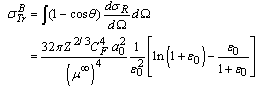(1)

With, C_F=0.8853414, and

Where , Z and E are the screened Rutherford cross-section, the transport cross-section, the atomic number of the atom target and the electron energy, respectively.

As is well known that the first Born approximation fails at low energies[3], the TCS () deviation reaches hundreds percent (%) for a number of elements compared to that obtained by quantum methods (see table 1 of the present work). However, the authors of[1] attribute eq. (1) to Jablonski with the following words: “ Jablonski[2] has then derived an improved analytical expression. In this derivation, the approximate analytical transport cross section, (denoted in the following) has been expressed by

”.

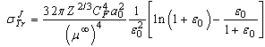We note that the index J in is denoted by[1]. However, the symbolization has used by Jablonski to denote the first-order Born approximation; he said[2]:” the index B denotes the first-order Born approximation.” In other words, Jablonski used the index B to denote “Born” whereas Rouabah et al[1] used the index J to denote “Jablonski”. Consequently, this incoherence needs to be corrected.

Actually, the TCS proposed by Jablonski lies in his paper[2]: “To obtain a more accurate analytical expression for , we need an additional analytical function correcting

(2)

With

(3)

where A₀ , A₁ , A₂ , A₃ , and A₄ are fitted constants for each element.”. Therefore the Jablonski transport cross section is given by (2-3) (cf. Eqs. (21) and (22) of[2]).

So, why has Jablonski completely changed the TCS expression? In other words, why didn’t Jablonski replace only one constant by a free parameter as Rouabah et al did? The answer lies certainly in reasons which will be discussed below.

2.2. The Analytical TCS Approximate of Rouabah et al.

Before quoting our overview points of this section, we recall that Rouabah et al used the same transport cross section expression given by (1) where the only difference is that has been taken as a free parameter. Thus to determine this one, they have adjusted -according to their notation- to Dapor TCS[4]). After a fitting process, they have suggested two interpolation forms of given by:

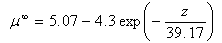(4)

(5)

The authors of[1] said: “Note that two forms (exponential and polynomial, respectively) have been here proposed for fitting the parameter versus z, leading to positron TCS - denoted and in the following which were respectively obtained using either Eqs. (1)-(4) or Eqs. (1)-(5)”.

3. The Confusion around the Interpolation Procedure followed by Roubah et al.

We have some questions about their fitting:

3.1. Is the Expression (1, 4) or (1, 5) Interpolate Well the Results Tabulated by Dapor[4]?

Rouabah et al adjusted their cross section given by (1) to that tabulated by Dapor[4], where is taken as free parameter. So, following an opposite reasoning, the authors of[1] stated explicitly that the results of[4] are in agreement with the eq. (1)! Before evaluating this statement, we noted that the authors of[1] did not give any explanation to their choice! We can see in fig.(2) of Jablonski’s paper[2] that the behavior is completely different from that obtained by quantum methods, particularly for heavy atoms cases (see figure (1) of the present work), whereas the right choose could the interpolation function from the shape of the tabulated values and not from the inverse. In the analytical expressions TCS reported in the literature take another form than that given by eq. (1) (see for example[5]). Indeed, Jablonski suggested an analytical TCS based on (1), but with another form (cf. Eq.(2)).

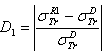
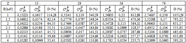
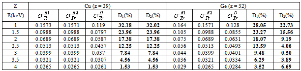
Table (1). Transport cross –section (in A2).      : First Born TCS given by (1).       Dapor TSC[4]. D: deviation between       and      .

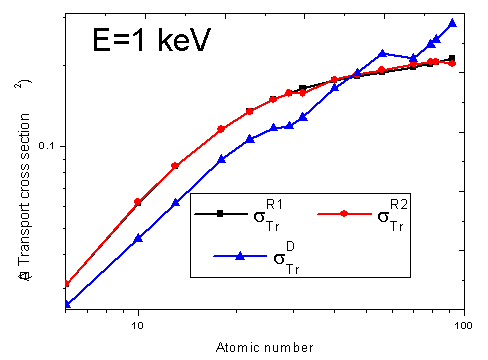Figure (1). The transport cross section(in A°2) in function of Z. : Rouabah et al TCS given by (1, 4)[1]. : Rouabah et al TCS given by (1, 5)[1]. Dapor TSC[4]

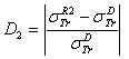
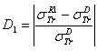
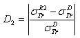
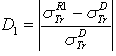
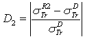
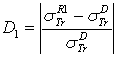
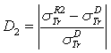
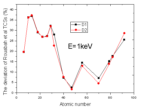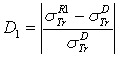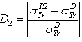Figure (2). The deviation (in %) of Rouabah et al results in function of the atomic number (Z). D1: the deviation between and . . D2: the deviation between and . . : Rouabah et al TCS given by (1, 4)[1]. : Rouabah et al TCS given by (1, 5)[1]. Dapor TSC[4]

3.2. How do They get through Z and E D Ependency of “μ^∞" to Solely Z?

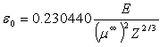
Rouabah et al[1] adjusted t o which is tabulated by Dapor[4]. Consequently, based on equation (1), we can easily conclude that "μ^∞" is given by:

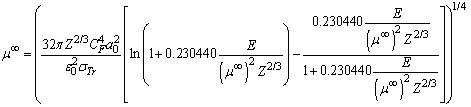(6)

Equation (6) shows clearly that μ^∞ is a function of Z and E where Rouabah et al[1] expressed it using one of the previous equations ((4) or (5)) which are dependent only on Z. They justified[1]: « These latter “(4) and (5)” have been determined for a large number of illustrative elements in the 1-4 keV energy range and expressed via the following expressions:

For 1 kev

For 2 kev

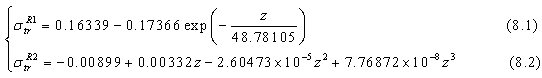For 3 kev

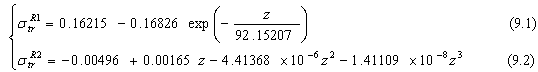For 4 kev

”.

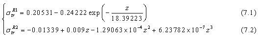
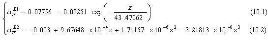Indeed, we consider the passage from equations (7-10) to equations (4-5) via the equation (6) is not evident. This remark will be shown as follows:

Let us take as example the next proof: when we replace by given by equation (7.1) at E=1 keV, in equation (6), we can resolve this latter (eq. 6) only for a known Z. Consequently, we should resolve the equation (6) for all given Z. Elsewhere, the above obtained results of will be different when we replace in equation (6) by given by equation (7.2) or other equations at different energies (i.e. at E=2, 3 or 4 keV). On other terms, we will find depending on the energy. However, their equations (4-5) show that depends only on Z, which is in contradiction with what will be expected.

3.3. Why didn’t Rouabah et al[1] Take into Account a Work with More Data Points?

Rouabah et al[1] have adjusted to the results of Dapor[4] represented in tabulated results only for selected elements. Elsewhere, the same author published a tabulated data for the differential, total and transport cross-section for all elements with atomic number Z from 1 to 92[6]. In addition, ELSEPA[7] allows the calculation of the differential, total and transport cross-section from 10eV to10⁹ eV and from Z=1 to 103. In other terms, more the data point number of the TCS as function of the energy (i.e “E_i, ”) increases more the interpolation could be more accurate.

3.4. Why didn’t Rouabah et al[1] Introduce the Energy Range up to 1 KeV in Their Study?

Let’s recall that the mono–energetic positrons beam, (regarding to the mean penetration depth with energies can be varied through the range up to 1 keV) allows to positron annihilation spectroscopy methods to be applied to study the surface and the nearest regions[8-9].

In addition, the authors of[1] said in their abstract that the information collected by their study could be useful for the evaluation of parameters required for “quantitative low-energy positron annihilation spectroscopy” (QLEPAS). After an attentive reading of their paper, we did not find any details about this point. In other word, what will be the interest of their fit[1] in the evaluation of parameters needed for (QLEPAS)? Therefore, we believe that more clarifications is needed.

In summary, Authors have not given any information concerning the relation between their fit and QLEPAS and in their interpolation they neglected an important domain where E<1 keV.

4. The Comparison of the Results Obtained by Rouabah et al. with other Works

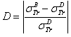
Before presenting this section, it is worth noting that among the most successful methods in determining the electron or positron differential cross-sections is the RPWEM (Relativistic Partial Wave Expansion Method)[10]. The differential cross-section obtained by using this latter (RPWEM) present a good agreement when compared with experimental data (see[11-12] and references therein). On other words the scattering cross section which could be measured experimentally is the differential cross-section. The total and the transport cross-section accuracy could be deduced by using the next definitions:

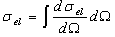(11)

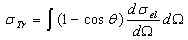(12)

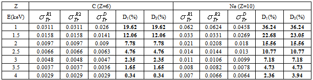
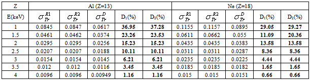
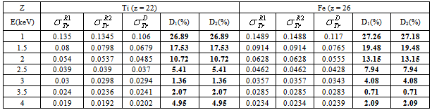
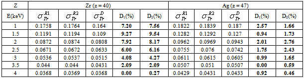
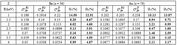
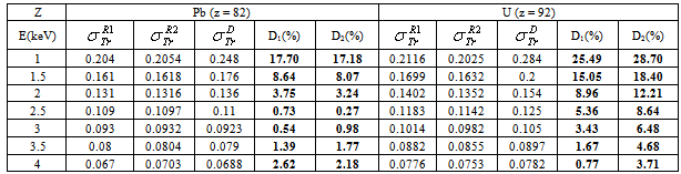
where and are the elastic total and the transport cross sections, respectively.

We note that Rouabah et al adjusted their cross section given by (1) to that tabulated by Dapor[4] who used the RPWEM. Tables (2-8) represent Rouabah et al TCS[1], Dapor TCS[4] and the percentage deviation between them. We think that, these deviations is clearly invalidates their proposal. The drastic deviation results could be observed also with other works based on quantum methods (see table (9) and ref.[13]).

N. B.: generally, if the aim of the work is to determine the best fit of tabulated data, the authors should propose an expression which agreed well with the data base. For example, the authors of[14] have suggested the backscattering coefficient as a function of the film thickness where the precision reached about 10^-8 (i.e. the percentage deviation reaches about 10^-6). We note that the authors of[10] implemented their model in Monte Carlo code with precision of their free parameters was less than 10^-10. Sometimes, despite the fact of the unsatisfactory data point number (which is not the case of[1]); the work will be considered only if the deviation is less than 5% (see for more detail as example[15-19]).

Remark: the authors of[1] presented six tables for their results even that it is an evident calculation (we think that one or two tables could be sufficient). Furthermore, we think that the authors of[1] presented two figures without any scientific argument (i.e. it is an additional fitting). Indeed, we think that the authors of[1] should present, in the figures (1) and (2)[1] their final results using equations (1, 4) or (1, 5) compared to[4] (i.e. not the intermediate or additional ones). In addition, the observed deviation (of ∼ 40 % at E=1 keV and ∼ 20 % at E=2 keV for some elements) is a proof on the invalidity of the work of[1] (for more detail, see figures (1) and (2) of the present work).

Table (2). Transport cross –section (in A°2) in function of Z.       : Rouabah et al TCS given by (1, 4)[1].       : Rouabah et al TCS given by (1, 5)[1].       Dapor TSC[4]. D1: deviation between       and      .      . D2: deviation between       and      .

Table (3). Transport cross–section (in A°2) in function of Z.       : Rouabah et al TCS given by (1, 4)[1].       : Rouabah et al TCS given by (1, 5)[1].       Dapor TSC[4]. D1: deviation between       and      .      . D2: the deviation between       and      .

Table (4). Transport cross–section (in A°2) in function of Z.       : Rouabah et al TCS given by (1, 4)[1].       : Rouabah et al TCS given by (1, 5)[1].       Dapor TSC[4]. D1: the deviation between       and      .      . D2: deviation between       and      .

Table (5). Transport cross–section (in A°2) in function of Z.       : Rouabah et al TCS given by (1, 4)[1].       : Rouabah et al TCS given by (1, 5)[1].       Dapor TSC[4]. D1: the deviation between       and      .      . D2: the deviation between       and      .

Table (6). Transport cross–section (in A2) in function of Z.       : Rouabah et al TCS given by (1, 4)[1].       : Rouabah et al TCS given by (1, 5)[1].       Dapor TSC[4]. D1: the deviation between       and      .      . D2: the deviation between       and      .

Table (7). Transport cross–section (in A2) in function of Z.       : Rouabah et al TCS given by (1, 4)[1].       : Rouabah et al TCS given by (1, 5)[1].       Dapor TSC[4]. D1: the deviation between       and      .      . D2: the deviation between       and      .

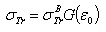
Table (8). Transport cross–section (in A°2) in function of Z.       : Rouabah et al TCS given by (1, 4)[1].       : Rouabah et al TCS given by (1, 5)[1].       Dapor TSC[4]. D1: percentage deviation between       and      .      . D2: percentage deviation between       and.

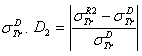
Table (9). Transport cross –section (in A2).       : Rouabah et al TCS given by (1, 4)[1].       : Rouabah et al TCS given by (1, 5)[1].       and       are the transport cross-sections calculated by[11] and[20] respectively

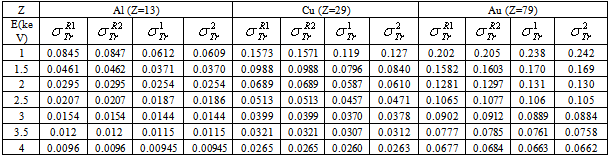
5. Conclusions

In summary, we have shown that Rouabah et al have not given any relation between their best fit and the parameters needed for the quantitative low-energy positron annihilation spectroscopy and they did not consider the energy interval where E<1 keV in spite of its importance in such study. Also, we have demonstrated that the transport cross section of Rouabah et al. is inaccurate and really it was not based on Jablonski’s expression[2].