-
Paper Information
- Next Paper
- Previous Paper
- Paper Submission
-
Journal Information
- About This Journal
- Editorial Board
- Current Issue
- Archive
- Author Guidelines
- Contact Us
American Journal of Condensed Matter Physics
p-ISSN: 2163-1115 e-ISSN: 2163-1123
2013; 3(3): 41-79
doi:10.5923/j.ajcmp.20130303.02
Study of Generation-recombination Processes by the Graph Theory
 Abstract
 Reference
 Full-Text PDF
 Full-text HTML
E. V. Kanaki1, S. Zh. Karazhanov2
1Physical-Technical Institute, 2B-Mavlyanova str., 700084, Tashkent, Uzbekistan
2Institute for Energy technology, 2027 Kjeller, Norway
Correspondence to: S. Zh. Karazhanov, Institute for Energy technology, 2027 Kjeller, Norway.
| Email: |  |
Copyright © 2012 Scientific & Academic Publishing. All Rights Reserved.
Generation-recombination (GR) processes of electrons and holes play important role in solar cells by controlling carrier lifetime and influencing on device performance. Commonly kinetic theory is used to study the processes. The aim of the article is to use graph theory and represent the GR processes in schematic form: defect states by dots and transitions between them by arcs. The centers of recombination have been classified within the definitions of the graph theory. An equation for the stationary distribution function of defects on states has been derived without constructing the system of kinetic equations. The theory can be helpful for simplification of the model of recombination through point defects. It should be based not only on smallest magnitude of the transition probability, but also on the role of the transition in the digraph of states. Distribution function of defects on their states has been found for asymptotic high injection level. We have derived the equation for the rate of the GR processes, which is universal for all types of point defects. Models of inertial and static behavior of the recombination centers have been discussed and the equations for them have been derived.
Keywords: Generation-recombination Processes, Charge Carrier Lifetime, Defects, Semiconductor Materials, Graph Theory
Cite this paper: E. V. Kanaki, S. Zh. Karazhanov, Study of Generation-recombination Processes by the Graph Theory, American Journal of Condensed Matter Physics, Vol. 3 No. 3, 2013, pp. 41-79. doi: 10.5923/j.ajcmp.20130303.02.
Article Outline
1. Introduction
- Graph theory was formed in XVIII century and its origin was related to mathematical puzzles. So, for a long time the doctrine about graphs was considered as a not serious topic because its practical applications were related only to games and entertainments. In this sense destiny of the graph theory can be compared to that of the probability theory, which initially was also considered with respect to games of chance. In XX century graphs have attracted attention of topologists and are considered as one of the chapters of topology, which was then one of the topics of mathematics and it interested only narrow range of readers. Since the time, there have been significant changes. Graph theory has been found to be important for solution of many problems of practice. The theory has found wide range of applications in different fields of science such as electrotechnics, electromechanics, radioelectronics, physics, chemistry, geodesy, sociology, economics etc. Literature on the topic increases with fastest rate (see e.g. Refs. 1-18).There are specialized journals such as “Journal of the graph theory”, and “Journal of graph algorithms and applications”. Specialized conferences are held on the subject. The reason for such a high interest to the graph theory can be explained by possibility of formulation and solution of problems in terminology and concepts of graphs, which are aggregation of dots connected with each other by lines. If the dots (vertexes of the graph) are identified as functional or constructional components and lines (arcs or edges of the graph) are identified as the cause and reason type relation, then the process or phenomena, system of equations or matrixes can be replaced by graphs, which consists of all the external and internal relations between objects of the phenomena or between variables in the system of equations. Such a graph model allows to establish clear relation between structure of the system and its quantitative characteristics, and to apply general methods to solution of the problems.
1.1. Applications of the Graph Theory
- Currently graph theory is widely used in many fields of science and technology. One of them is programming7-10. Here there is an important problem of segmentation of programs to minimize exchanges between the operative and external memories. In graph theory the problem is related to decomposition of graphs. Another problem of optimal distribution of different program blocks requires minimization of expected number of transfer of controlling, which can be solved by constructing the Hamilton cycle in the graph theory. Also, there are some other problems such as itinerary, modelling of the data transfer and distribution of information in the communication systems, which can be solved using the graph theory.Automation of designing of the microelectronic computational structures and systems can also beconsidered from the point of view of the graph theory. In the topic related to recognizing of the graph isomorphism, finding all of the ways, optimal decomposition of the graphs, construction of the minimal connecting trees etc are very important.Graph theory has found an application also in description of mechanical movement of matter (see e.g. Refs.11, 12). It is found to be a convenient tool for presentation and construction of the system of equations. Graph models have been found for systems described in terminology of energy and power, which include the Lagrange equation and generalized coordinates. The models allow to understand both energetic structure of a system and its functional behaviour including non-linearity and to withdraw the equations in the state space. In hydrodynamic systems graph theory allowed to replace description of hydraulic systems with distributed parameters with those of point ones13. In geodesy14 it allowed to make topological classification of geodesic constructions and to find possibility of description of the geodesic network structure by the Boolean algebra. Graphs have also been used for construction of models of the human-heart-vessel system with distributed parameters15. The models include the heart, arterial, capillary and vein parts of both system and lung blood circulation. Due to universality of the graph theory language, the models are functionally soft and can be modified. One of the models is body movement caused by blood flow of human mechanically separated from the earth. It provides the possibility for indirect determining the characteristics of the heart operation.Electrical network can be described as aggregation of elements and nodes connecting the elements. It can be abstracted to the concept of graphs of electrical networks with multipole elements. Basic concepts of the mathematical graph theory for such graphs have already been developed, which have found application in analysis of networks by topological methods16. Mathematical tool of the scheme multiplicities, introduced for description of graphs, provided formalization of the procedure for analysis alleviating construction of its algorithm and further improvements in computational designing of electrical networks.Graph theory is actively used in chemistry, biology and physics (see e.g.Refs. 17, 18). If atoms are presented as vertexes of a graph and lines connecting the vertexes as relations between them, then one gets the graph presentation of molecular or crystal structure of matter. This is the well-known classic language of structural chemistry and crystallography.Denoting the matters by dots and reactions between them by lines, one comes to graphical presentation of chemical reactions, widely used in chemistry, biology and physics 17-20. Similarly, if dots correspond to defects and lines to the defect transformations, then one can get the photo-, thermal- and recombination-stimulated defect reactions21well known in modern solid state physics. If dots identify the different charge or configuration states of defects and lines identify defect transitions between the states, such a graph describe GR processes in semiconductors22-27. If variables are depicted by dots and relations between the variables by lines, then one gets the system of linear equations describing the chemical, biological or physical etc system. Often the reaction schemes have been depicted without knowing that this is the graph of the complicated phenomena. Conception of the scientific field “Synergetics” appeared at intersection of many other fields such as chemistry, biology, physics etc resulted in the necessity to study complex behaviour of non-linear dynamic systems. The problem was to define the mechanism and parameters, which are responsible for spontaneous formation of multiple stationary states, periodic and chaotic oscillations in point and distributed systems. Graph theory has found application in this field also17, 18. Distinct from graphs of linear systems, which identify vertexes as matters and arcs as reactions, graphs of non-linear phenomena systems are bipartite, which contains two types of vertexes: matters and reactions. Arcs (or edges) of a bipartite graph indicates that some matter is formed or expended during the reaction. In the above-listed kinetic problems, graph theory provided the possibility to find stationary concentration of intermediate matters, stationary velocity of complicated reaction, to write down the characteristic polynomial, which is necessary in studying the relaxation processes, and to analyse the number of independent variables of the stationary kinetic equations etc.17, 18.Solution of many problems in chemistry and physics of polymers is simplified significantly if they are formulated in terminology of the graph theory17. It is especially effective in consideration of the branched polymers28, 29. Note that application of graph theory is not limited to the above list. Further, we will concentrate attention to GR processes.
1.2. Motivation in Using the Graph Theory for the Study of Generation-recombination Processes
- As different schemes, matrixes, systems of equations are used in investigation of GR processes, graph theory, which studies topological properties of schemes, can find application in this field also. Together with the usually used kinetic approach it can be a new effective theoretical tool in this field. It is interesting not only because of its novelty in applying in GR processes, but also due to its importance in simplification of the system of kinetic equations, finding asymptotical values of the distribution function, and because it has brought us to new results. It is not a principally new method, but it amplifies significantly and extends the kinetic approach leading the GR processes to maximal formalization. Application of the graph theory in this field allows to present the results analytically and to supply with topological picture of the relations between variables, which in some cases can lead to new results.Earlier, we have reported our preliminary results about using the graph theory in investigation of GR processes 26. In addition to it, in the present article we found more interesting results, which demonstrate power of the graph theory as a new mathematical tool and its prospects in physics of semiconductors. In addition to the kinetic approach, graph theory can be an effective tool for analysis and solution of a number of problems.As the graph theory is not well known to wide range of readers in the field of physics of semiconductors and currently there are no systematic studies on application of the theory to GR processes, the authors pursue the following goals: (i) to acquire specialists in the field of physics of semiconductors with basic concepts of the graph theory, with its methods, definitions and terminology; (ii) to demonstrate on examples how the theory can be used for GR processes and to present the results obtained systematically. The most serious limitation of this paper is that it covers consideration of only point defects. Recombination through linear and bulk defects, nanosized objects, Boltzmann kinetic equations are not considered. These limitations emphasizes importance and actuality of the results presented in this review.During study of the graph theory our attention was turned to search of possibility of direct application of existing solutions and basic concepts of the graph theory to problems of GR processes. Therefore, some definitions and theorems have been used without proof and justification, referring to corresponding sources. Upon presentation of the results, usual terminologies of the graph and recombination theories have been used. So, no preliminary knowledge of the graph theory is required, since all necessary ones are in the paper.
1.3. GR Processes Through Point Defects
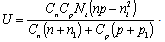
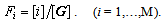
- Prime task in investigation of influence of defects on physical properties of semiconductors is finding the distribution function of defects on states and GR rate, which depend on temperature, carrier injection, illumination, etc. This is because many electrical properties of semiconductors, in particular, specific (photo-) conductivity, carrier recombination rate and lifetime, intensity and spectral distribution of luminescence, depend on the number of defects in that or other state. Usually for this purpose, system of kinetic equations for free carrier and defect concentrations is constructed (see, e.g.,Refs.22,23,30-36). By solving the system, one can get the required distribution function and recombination rate.Theory of the GR processes in semiconductors is first developed by Shockley-Read32 and Hall31 for the simplest defect with one energy level in the band gap and two charge states. Since then the theory has been extended for more complicated models of point defects: multiple charge defects without excited states32-34, two-charged defects with one excited state22,34,36, four charge defects without excited states and three-charged defects with an excited state24,37-40, bistable defects41, hypothetical model of metastable defects42. First systematic investigation of the GR problem is done in the book by Landsberg22. The above studies are based on kinetic theory, which is easy to use for simple defects with two or three states in the band gap. However, it is more complicated for defects with more number of charge states and different number of configurations and/or excited states. Analysis of literature shows that many semiconductors may containdifferent types of complicated defects, which modulate carrier lifetime and electrical properties of the material. Some examples for Si are, e.g., boron-oxygen complex Si43, donor-H complex44, which are responsible for degradation of carrier lifetime in solar cells, metastable oxygen - silicon interstitial complex in crystalline silicon45, metastable and bistable defects46, etc. Theoretical analysis of such system by using the kinetic theory might become a time consuming work and having an alternative method is important. Also, the rate of GR processes is commonly estimated by equation

 , where
  and
and  are the excess electron(hole) concentration and lifetime, respectively, which can be measured experimentally. Here, the approximation
 has been derived from the theory by Shockley-Read30 and Hall31. However the question as to whether the equation is valid for all models of recombination through point defects is open. In this article, we will use graph theory and solve these challenges. Applying a new method for study of a process always is interesting and might lead to some exciting results. In particular, by using the graph theory we have approached the GR processes from different angle.
 2. Methods
2.1. Assumptions
- The defects can be in different charge states or configurations. The origin of the defects can be different: intrinsic, extrinsic defects, or their complexes. The defect can have any number of configurations and charge states. The defects should be independent each from other. They should not interchange by carriers by tunnelling and should not interact through electrical and magnetic fields or mechanical stresses of a distorted lattice. It is assumed that the semiconductor is non-degenerate and that influence of GR processes determined by materials properties such as the band-to-band or Auger recombination can be neglected. Stationary state of the system is suggested to be stable. Dynamic equilibrium is assumed in the transitions between different states. Also, we did not account for the processes of defect generation, annihilation, and migration.
2.2. Kinetic Theory
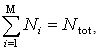
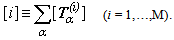
- Kinetic theory stands22 at the very heart in the study of the GR processes taking place via, in particular, point defects of net concentration Ntot. The defect is supposed to be in i=1, …, M states with the concentration Niin the i-thstate, so that M>Ntot[Fig. 1]. Transition from one state, i, into another one, j, is denoted as
 characterized by the weight, ωij, which is equal to the probability of the transition per unit time. Kinetics of the concentration of the defects can be described by the following equations
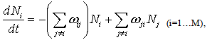 | (1) |
 | (2) |
 to be called hereafter as the stationary distribution function
 | (3) |
 | (4) |
 | (5) |
 | (6) |
 and
and  are the excess concentrations,
  are the net concentrations, and
  and
and  are the equilibrium concentrations of free electrons and holes. The relation between them can be found from the electro-neutrality requirement
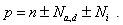 | (7) |
 stands for the concentration of shallow acceptors and donors, respectively.
  is the concentration of the recombination center. The (+) sign comes if the defect is negatively charged and (-), if it is positively charged.
2.2.1. Theory of Recombination by Shockley-Read-Hall
- One of the examples we consider is the theory developed by Shockley and Read30 as well as by Hall31 (SRH). In the theory transformations of the defect from one charge state into another one can be denoted as 1
 2 and 2
 1 (Fig. 1(a)). Each of the transitions
  in the Fig. 1(a) have been marked by corresponding weight ωij
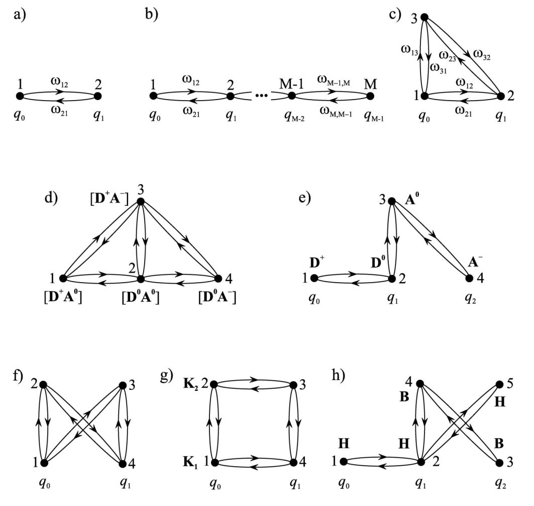 | Figure 1. Digraphs of states for defects with (a) two-charge and (b) M-charge without excited states, (c) two-charge defect with one excited state, (d) donor-acceptor pairs with three different charge states, (e) three-charge defects with one excited state, (f) two-charge defect with two excited states, (g) two-charge bistable defect and (h) three-charge U‾-centers in n-Si. Each vertex of the digraphs corresponds to a particular quantum state of the defects and arcs correspond to the allowed transitions between these states. Weights of the transitions ωij are equal to the probabilities of the corresponding transitions per unit time. Vertices of a digraph, posed along one vertical, concern to the same charge state of a defect. The lowest vertex corresponds to the ground state whereas the highest ones denote excited states. The digraphs are symmetric, which means that transition described by the arc  of the digraph contains its counter arc j of the digraph contains its counter arc j i. Also, the digraphs are strong, which means that all their vertices are mutually accessible i. Also, the digraphs are strong, which means that all their vertices are mutually accessible |
 | (8) |
 and
and  are the specific probabilities of carrier capture by the defect and of emission from the defect level into the allowed bands. The fraction
  of a defect with an electron and recombination rate
  found from Eqs. (1)-(6) at steady state conditions are at the form
 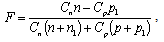 | (9) |
 | (10) |
2.2.2. Theory of Recombination ViaBistable Defects
- Upon transitionsof bistable defects 1
 3 and 2
 4 (Fig. 1(b)) the charge of the defects is conserved and the defect configuration changes, whereas upon 1
 2 and 3
 4 the charge state of the defect changes without changing of the configuration. The other possible transitions 1
 4 and 2
 3, which would be accompanied by transformation of both configuration and charge, have been neglected. The reason is that we have not seenany experimental evidence for existence of such bistable defects in Si. Weights of each of the transitions
  denoted by ωij[Fig. 1 (d)] are
 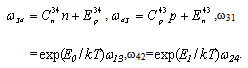 | (11) |
 3 and 2
 4, respectively. E0 and E1 are the activation energies of configuration transformations of the defect without an electron and that with an electron, kT is the thermal energy.
2.3. Elements of the Graph Theory
- The following definitions might be important to link the graph theory with the generation recombination processes through the ensemble of identical and independent from each other point defects, which can be in M different quantum states
 (i= 1, …, M). These definitions can be found in Refs.1-3, 5-7, 11, 12, 17.Definition 1. A graph is a mathematical structure composed of points called vertices, which are the fundamental building blocks of graphs. The vertices are connected by lines called edges or arcs. In GR processes each state
  of a defect (i= 1, …, M) corresponds to a vertexi of the graph. The arc, connecting the defect states iandj, indicates an allowed tra
 nsition from the state
  to the state
 probability of the transitions between the states
  and
and  per unit time corresponds to the weight ωij ([T1]) of the arc
  . If there are several competing mechanisms of transition of the defect from the state
  to the state
  one can draw several arcs coming out from the vertex i to the vertex j, thus forming the so-called multiple arcs1-4. Each of the arcs should be assigned the weight
 , which is equal to the transition probability by the corresponding mechanism “α”. There might exist also loops, which are the arcs going out of a vertex and coming back into it without connecting to any other vertex. Existence of a loop indicates the possibility of static influence of defects on electronic transitions in the system, which we will discuss later. Some mechanisms of static involvement of defects are below. Definition 2. The defect states and transitions between them have been presented pictorially, which we call the digraph of states G.There are two types of graphs: undirected graph, consisting of unordered vertices with a set of edges and directed graph, which consists of ordered vertices and a set of edges. A digraph G can be said to be strongly connected if all its vertices are mutually reachable. Important feature of the strong digraphs is that for each its vertex there exist at least one directed tree covering the digraph and growing into this vertex. Physically it means that the defect state in any state i (i= 1,…,M) can reach any of the other states. Fig.1 presents examples of such strongly connected digraphs. The case of weakly connected digraphG will be considered separately. Definition 3. One of the widely used definitions in the graph theory is called tree, which is an undirected graph in which any two vertices are connected by exactly one simple path. In other words, any connected graph without cycles is a tree. A forest is an undirected graph, all of whose connected components are trees; in other words, the graph consists of a disjoint union of trees. A directed tree is a directed graph which would be a tree if the directions on the edges were ignored. Some authors restrict the phrase to the case where the edges are all directed towards a particular vertex, or all directed away from a particular vertex. A tree is called a rooted tree if one vertex has been designated the root, in which case the edges have a natural orientation, towards or away from the root. Definition 4. The directed tree T(i) covering the M-vertex digraph G and growing into its vertex i is defined as the subgraph in G which includes all the M vertexes and (M–1) arcs in such a manner that starting from any vertex other than i and moving along these arcs one necessarily comes into the vertex i (to be called “the root” of the tree T(i)). To show that the results of the kinetic approach can easily be obtained using the graph theory, we will analyse the kinetic equations (1) and (2), describing the kinetics of distribution of defects on their states. Since the defects comprising the ensemble are assumed to be independent, the probabilities of transitions ωij do not depend on Fi explicitly. Therefore, from the mathematical point of view the Eqs (3)-(4) are the system of linear inhomogeneous equations for Fi (i= 1,…,M). Such a system of equations can be solved by the graph theory. Below we show that the solution of this system of equations can be constructed with the help of a digraph of states G. We will consider a strongly connected digraph G with vertices, which are mutually reachable. In Fig. 2 we show example of an eight-vertex digraph G with loops 4
 4 and 5
 5 and multiple arcs 4
 1 and 2
 5 and covered with a tree T(1)=(5
 2
2 1)&(3
1)&(3 1)&(6
1)&(6 4
4 1)&(7
1)&(7 4)&(8
4)&(8 4) that grows into the vertex 1. If there are several trees covering a digraph G and growing into its vertex i, a subscript is used in the notation
  to distinguish them each from other. The trees are considered as different when the sets of their arcs do not coincide. Each tree
  will be assigned the weight
  , which equals to the product of the weights of all its arcs:
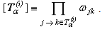 | (12) |
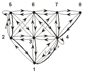 | Figure 2. The digraph G. One of the trees T(1) is selected that covers the digraph and grows into the 1st vertex. Arcs not included into the tree are plotted by dots. The tree T(1)=(7 4)& (8 4)& (8 4)&(5 4)&(5 2 2 1)&(3 1)&(3 1)&(6 1)&(6 4 4 1) consists of seven arcs linking all eight vertices of the digraph G in such a manner that, moving along these arcs from any vertex, one inevitably comes into the root vertex 1 and leaving the vertex is not possible. This example shows the important features of “growing into” type trees. It has no bifurcations, i.e. there are no groups of two or more arcs issued from the same vertex. It does not contain cycles, including loops. Deleting any arc from a tree, but saving all its vertices, leads to breaking of the tree into two fragments, which are also the growing into type trees. Thus, if the arc 4 1) consists of seven arcs linking all eight vertices of the digraph G in such a manner that, moving along these arcs from any vertex, one inevitably comes into the root vertex 1 and leaving the vertex is not possible. This example shows the important features of “growing into” type trees. It has no bifurcations, i.e. there are no groups of two or more arcs issued from the same vertex. It does not contain cycles, including loops. Deleting any arc from a tree, but saving all its vertices, leads to breaking of the tree into two fragments, which are also the growing into type trees. Thus, if the arc 4 1, e.g., is excluded from the tree T(1), then one can get the trees (5 1, e.g., is excluded from the tree T(1), then one can get the trees (5 2 2 1)&(3 1)&(3 1) and (6 1) and (6 4)&(7 4)&(7 4)&(8 4)&(8 4) growing into the 1st and 4th vertexes, respectively. Note that the sole vertex may be considered as a trivial case of the trees. The addition to a tree covering a digraph G of one more arc of G creates a cycle and/or a bifurcation. For example, if T(1) will be added with the arc 1 4) growing into the 1st and 4th vertexes, respectively. Note that the sole vertex may be considered as a trivial case of the trees. The addition to a tree covering a digraph G of one more arc of G creates a cycle and/or a bifurcation. For example, if T(1) will be added with the arc 1 2, then the cycle C = 1 2, then the cycle C = 1 2 2 1 will appear with two trees growing into its vertices: 5 1 will appear with two trees growing into its vertices: 5 2 and (6 2 and (6 4)&(7 4)&(7 4)&(8 4)&(8 4 4 1)&(3 1)&(3 1). Such constructions are known as the functional graphs 1). Such constructions are known as the functional graphs |
 | (13) |
 | (14) |
 | (15) |
3. Results. Non-Equilibrium Distribution Function
3.1. Classification of Recombination Centers According to the Graph Theory
- As noted earlier, recombination centers can be in several states differing each from other by charge and excited states or configuration and transition between them is possible during GR processes. By one vertex corresponds to each state of the defect. Below we will perform classification of the recombination centers according to the graph theory, which is based on the total number of states the defects.
3.1.1. Defects with two Charge States: Bivertex Digraph
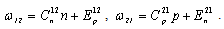
- The simplest type of defects can be in one of the two charge states: neutral and positively charged or neutral and negatively charged. Theory of recombination through such defects was developed by Shockley and Read 30, and Hall 31 for non-degenerate case and without accounting for the Auger effects. Digraph corresponding to such a defect is shown in Fig.1 (a) and can be called as bivertex digraph. The vertex 1 corresponds, for example, to the defect in charge state q0 without an electron whereas the vertex 2 corresponds to the defect with one trapped electron and having, therefore, the charge q1= q0– 1. If one neglects the multi-particle mechanisms of transitions the probability ω12 of capture of an electron by the defect and probability ω21 of emission of an electron from the defect are: ω12= Cnn+ Ep and ω21= Cpp+ En. One can take the mechanism of Auger recombination into account by incorporating the terms like
 nξpζ into the probabilities ωij; in non-degeneracy case the parameters ξ and ζ are integers and are equal to the number of free electrons and holes participating in the transition, respectively (see, for example, 22). In the degenerated case the parameters can be fractional 47; the coefficients
  [L3(ξ+ζ)T1] are determined by the nature of a defect and its electronic states, and also by mechanisms of energy dissipation.
3.1.2. A Defect with net M-charged States Without Excited States: M-vertex Digraph
- The digraph, corresponding to a defect, which can be in multiple charged states and does not have excited states, is shown in Fig.1b. It can be called as M-vertex graph with M vertices corresponding to different charge states. The i-th (i= 1,…,M) vertex is supposed to correspond to the defect with (i–1) captured electrons, so that qi = qi–1– 1. Charge of the defect in the state 1 is designated as q0. In non-degenerate case upon neglectingthe multi-particle effects the transition probability of the defect from the state iinto the state i+1 is determined by the probabilities of capture of an electron from the conduction and valence bands ωi,i+1=
 . For reverse transitions it is defined by probabilities of departure of an electron into allowed bands: ωi+1,i =
  (i= 1,…,М–1). GR processesvia such defects were studied32,33,35by the kinetic theory.
 3.1.3. A Defect with Two-charged and One Excited States: Three-vertex Digraph
- Such a defect can be in two charged states. In one of them it has one excited state. In graph theory such a defect can be plotted as a three-vertex digraph [Fig.1c]. The vertices 2 and 1 correspond to the ground states of the defect. In one of them it contains one electron, in the other state it has no electron. The vertex 3 corresponds to the excited state with the same charge as the state 1.Then the transitions 1
 3 correspond to the intra-center ones. Distinct from other transitions, charge state of the defect will not be changed. Theory of GR processes through such defects, when the excited state is an exciton bound to a defect has been studied in Ref.[34]. Similar model was proposed in correlation mechanism of recombination36.
 3.1.4. Defects Described bythe Four-vertex Digraphs
- Defects, which can be in four-charge states without excited states can be described by the four-vertex digraph. It can be regarded as a particular case of the multiple charged defect described in Subsection 3.1.2 for when M=4. Below we list some examples of such defects. One of them is the defect with three different charged states and with one excited state. The other one possesses two charged states with one excited state for the each charge state or both excited states at one of the charge states. Donor-acceptor[DA] pair consisting of closely situated donor (D) and acceptor (A)centers with allowed electronic exchange between D and A can the third example of the three-charge defect with one excited state. The fourth example is the solitary pair, which cannot influence on each other because of large distance between them. The appropriate digraph is shown in Fig.1d. The vertex 1 corresponds to the positively charged pair[D+A0]. The vertices 2 and 3 are the neutral states of a pair[D0A0] and[D+A‾] respectively. The vertex 4 is a negatively charged pair[D0A‾]. Transitions between the states 2 and 3 are the intra-centers ones, whereas other transitions are the carrier exchange between the components of the pair and allowed bands. One more example of the defects with three-charged states and one excited state is the U‾-center40. Digraph for the defects is shown in Fig.1e. Vertex 1 is the positively charged state, which is designated as D+ in [Ref.40]. Vertex 2 and 3 correspond to the neutral states of the defect D0and A0, which differ each from other by the configuration. Vertex 4 are the negatively charged state of the defect A‾. Transitions 2
 3 between the neutral states D0 and A0 correspond to the transformation of the configuration of the defect whereas the remaining transitions are the electronic exchange of the defect with allowed bands.Theory of recombination through defects with two charges in the ground and excited states was studied in Ref. [37]. Afterwards the model of cascade recombination was studied in a number of other papers22. Fig. 1f presents digraph for the defect with two charge states. The defect in its empty ground state 1 can capture an electron from the conduction band into the upper level, and be transformed into the filled excited state 3. From the state it can relax into the ground state 4, filled with two electrons. Being in this state it gets the possibility to capture a hole into the lower level, located closer to the top of the valence band, i.e. to pass the electron with smaller energy to the valence band and to move thus into an empty excited state 2. Then it can be transformed into the state 1 due to transition of an electron from the upper to the lower level of the defect. Together with the above-mentioned transitions reverse transitions have been taken into account.Recombination theory through the two-charge bistable defects with one excited state for each charge state is described inRefs. [41,48]. It should be noted that many defect complexes in Si such as, e.g., FeiBs, FeiAls, FeiGas, FeiIns, B-O, etc. are the examples of the bistable defects. Digraph for the defects is shown in Fig.1g. Vertices 1 and 2 correspond to the empty defects with charge q0 in space configurations Q1 and Q2. The vertices 4 and 3 correspond to the defects in the same configurations with an additional electron and, therefore, with the charge q1 = q0 – 1. For such a defect in silicon, for example FeiAls, the two charge states are Fei2+Als‾ and Fei+Als‾ in two possible orientations along the direction <111> and <100> (Ref.[49]). Therefore, the transitions 1
 2 and 3
 4 are the transformations of the configuration of the defect without charging the charge state, whereas 1
 4 and 2
 3 are accompanied by carrier exchange of the defect with allowed bands, but without changing the reconfiguration. Note that changing the charge state of a defect simultaneously with its configuration (i.e. transitions immediately between the states 1 and 3 or 2 and 4), is considered as improbable event and in Ref.41 it was not taken into account.
3.1.5. Defects with Five States: Five-vertex Digraph
- There are several types of defects, which can belong to the five-vertex graphs. One of them is the defect, which can be in five charged states and without excited states. The other one is the defect with two charge states and three excited states. Below we will focus on an example of the defect with threecharge and two excited states49 in the study of the U‾-centers. Hydrogen and thermal donors in Si can be regarded as examples. The digraph of states is shown in Fig.1h. The defect in the state 1 is double positively charged (q0 = +2). By capturing an electron it passes into a single-charged state 2 (q1 = +1). From the state it proceeds either into the state 4 with the same charge q1 but in another configuration, or, by capturing an additional electron into the neutral state 5 (q2 = 0). In the state 4 the defect can capture an electron and proceed into the neutral state 3, which differs from the state 5 by space configuration. In Ref.[49] configuration of the states 4 and 3 are identical (designated as “B-configuration”) and that of the states 1, 2 and 5 are also identical (“H-configuration“). So, the transitions between the states 2 and 4 are related to change of configuration of the defect whereas the remaining ones are accompanied by changing of charge state of the defect because of the electronic exchange between the defect and allowed bands occurring without changes of the configuration.
3.2. Distribution of Defect Concentration on States: Digraph of States
- As mentioned above, at steady state conditions the portion of defects Fi in the i-th state can be estimated as the specific tree-weight of the i-th vertex of the digraph G[Eq. (15)]. The Eq. (15) can be immediately deduced from the matrix-tree theorem proved2 by W. Tutte[Appendix A] without constructing the system of kinetic equations. We shall also reveal the informal aspect of the result by showing that it is only the tree form of the state weights[Eqs. (12) and (13)] that is capable of providing the balance of flows in the stationary system at arbitrary variations of transition probabilities. So, by the tree-weight rule[Eqs. (12)-(15)] it becomes possible to obtain Fi from the digraph of defect states G. First of all, let us give the comprehensive description of structure of the equation for Fi. From the properties of a M-vertex tree T(i) growing into the i-th vertex it follows that its weight[T(i)][Eq. (12)] consists of (М–1) terms ωjk. Among them there are no weights with equal indexes ωjj, since the tree has no loops i
 i, no products of weights with equal values of the first index like ωjkωjl, since the tree of the “growing into” type has no bifurcations like (j
 k)&(j
k)&(j l) and, no factors with cyclic values of indices, i.e. the factors like ωjkωkj, ωjkωklωlj, etc., since the tree has no cycles like j
 k
k j), (j
 k
k l
l j, etc. Under these conditions being fulfilled, among the values of the second index of the factors ωjk there will necessarily be such a one, which is not among the values of the first index and this is the value which corresponds to the root vertex i of a tree T(i). For example, the product ω52ω21ω31ω64ω41ω74ω84in Fig. 2 fulfils all the above requirements and hence represents the weight of the tree with eight vertices, which grows into the 1st vertex. The product consists of the seven terms ωij. Based on this equation one can easily get the visual image of the tree: since it consists of the weights of the arcs 5
 2, 2
2, 2 1, 3
1, 3 1, 6
1, 6 4, 4
4, 4 1, 7
1, 7 4 and 8
 4, we deal with the tree Τ(1) = (5
 2
2 1)& (3
 1)&(6
1)&(6 4
4 1)&(7
1)&(7 4)&(8
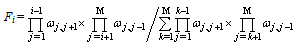
4)&(8 4) that has been depicted in Fig.2. So, the above description fully determines the structure of each addend in the numerator and denominator of the Eq. (6). Number of addends in the numerator in Eq. (6) depends on features of the scheme of allowed transitions and can be found with help of the square matrix K =
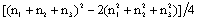
  of order M. Each diagonal element kii of the matrix is equal to the number of arcs issued from the vertex i and the off-diagonal element kij (i≠j) is equal to the number of arcs coming from the vertex j into the vertex i taken with minus sign. Loops of the digraph G are not taken into account. Cofactor of any element in the i-th column of the K-matrix gives the number of the trees covering G and growing into the i-th vertex (see, e.g., Ref. [1]). It gives the number of addends in the numerator in the equation for Fi. Number of addends in the denominator of the Eq. (15) is equal to the total number of addends in the numerators for all i= 1,…,M.From the above description it is seen that the structure of Eq. (15) for Fi bears a strong resemblance to the equation for the probability of a complex event which may happen by several mutually exclusive ways. Each way consists of a few independent steps: each such step is a certain transition of a defect from one state into another one, and each way is a bunch of the transitions forming a certain tree. So the weight of the tree
  is the probability of reaching the final state i by the certain “way”
  , which is the product of the probabilities of “steps” ωij constituting this “way”; the denominator[G] in Eq.(15) is simply a normalizing factor. Unfortunately, we failed to find the physical reasons for this remarkable resemblance. The GR processes fulfil the principle of detailed balance, i.e. obey the Gibbs statistics. It means that at thermodynamic equilibrium case each transition of a defect from the state i to the state j described by the arc i
 j is balanced by reverse one corresponding to the arc j
 i. By other words, the GR processes of electrons and holes through point defects should be described by symmetric digraphs having the arcs i
 j and j
 i at the same time. The weights[i]eq must obey to the Gibbs statistics and the following relationship should be fulfilled:
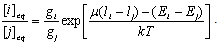 | (16) |
 j and j
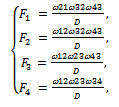
 i, is a root of ММ–2 trees, where M is the number of the vertices. Let us examine the digraphs in Figs.1a,b,e,h with acyclic bases. In particular, base of the digraph in Fig. 1h is an undirected tree (1—2—4—3)&(5—2) and have therefore only one tree growing into each of their vertices. Fig. 3 shows the spanning trees growing into the 2nd vertex of the digraphs of Fig. 1. Figs.3a,b,e,h show those trees growing into the vertex 2. For this reason, the stationary distribution function for these models can be constructed. For example, for bivertex digraph G[Fig.1a]
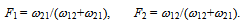 | (17) |
 1) of the weight[Τ(1)] = ω21 grows into the vertex 1. Therefore the tree-weight of this vertex is[1] = ω21. Similarly, tree-weight of the vertex 2 is[2] =[Τ(2)] = ω12. In particular, assuming ω12 = Cnn+ Ep and ω21 = Cpp+ En, one can get the common result of Shockley-Read-Hall recombination theory30,31. To get a more general result for multiple charge defects without excited states one should deal with the M-vertex digraph G shown in Fig.1b. Vertex i of the digraph is a root of the only tree Τ(i) = 1
 2
2 …
… (i–1)
(i–1)  i
i (i+1)
(i+1)  …
… (M–1)
(M–1)  M with the weight
 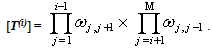 | (18) |
 | .(19) |
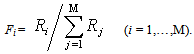
 and introduces the notations
 | (20) |
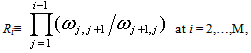 | (21) |
 | (22) |
 | (23) |
 | (24) |
 trees. Therefore, three, four and eight trees grow into each vertex of the digraph in Fig.1c,f,g, and d, respectively. Having constructed all the trees for a digraph one can write down the equation for the distribution function. For example, in Fig.3four covering trees
  grow into the 2nd vertex of the digraph G[Fig.1g]. The trees have the following weights:
  ω12ω32ω43,
  ω14ω43ω32,
  ω41ω12ω32,
  ω34ω41ω12. Hence, the tree-weight of the 2ndvertex is[2] = ω12ω32ω43 +ω14ω43ω32+ω41ω12ω32+ω34ω41ω12. Tree-weights of the other vertices are:[1]=ω43ω32ω21+ω23ω34ω41+ω32ω21ω41+ω34ω41ω21, [3] =ω12ω23ω43 + ω14ω43ω23 + ω41ω12ω23 + ω21ω14ω43, and[4] =ω12ω23ω34 + ω14ω23ω34 + ω32ω21ω14 + ω21ω14ω34. AccordingtoEqs. (14) and (15) the distribution function is:
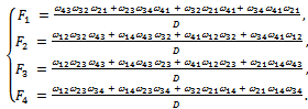 | (25) |
 j and j
 i and if the transitions are the only paths linking the states, then the rates of transitions between the two states will be balanced not only in equilibrium but also in non-equilibrium stationary state: Fiωij=Fjωji. Arcs corresponding to the transitions are known as bridges in the digraph G: removal of these arcs will cause splitting of the digraph G into two disconnected fragments. One can easily prove it if notes that when there is only one path i
 j between the vertices i and j. Then any tree growing into the vertex i can be obtained from some tree growing into the vertex j by reorientation of the arc i
 j into j
 i and vice versa. Hence, weights of these vertices satisfy the Eq. [i] =[j]ωji/ωij. Then applying the Eq.(15) one obtains proof of the above statement. Dueto this fact ‘the principle of non-equilibrium detailed balance’ will be fulfilled for any states of a system in steady state described by symmetric strong digraph with an acyclic base (see, e.g., Figs.1a,b,e,h).
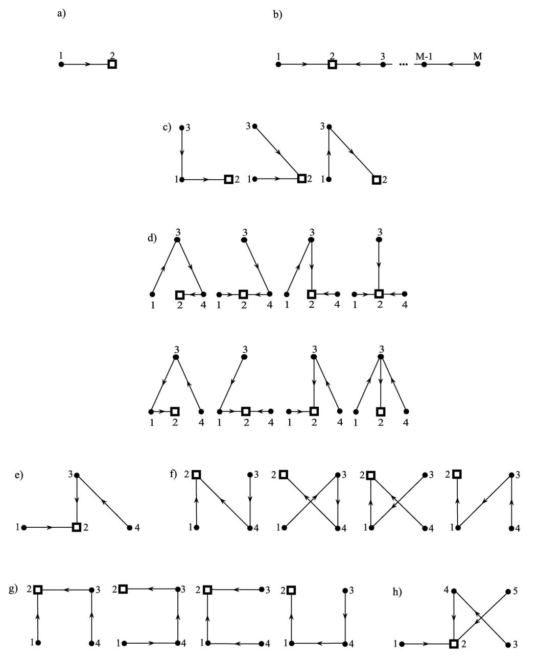 | Figure 3. Spanning trees growing into the 2nd vertex of the digraphs in Figure 1: for defects with (a) two-charge and (b) M-charge without excited states, (c) two-charge defect with one excited state, (d) donor-acceptor pairs with three different charge states, (e) three-charge defects with one excited state, (f) two-charge defect with two excited states, (g) two-charge bistable defect and (h) three-charge U‾-centers (four covering trees  grow into the 2nd vertex. The root vertex 2 is denoted as a square. Each of the trees makes a contribution to the tree-weight of the 2nd vertex of the digraphs grow into the 2nd vertex. The root vertex 2 is denoted as a square. Each of the trees makes a contribution to the tree-weight of the 2nd vertex of the digraphs |
3.3. Graph Theory in Simplifications of the Scheme of Electronic Transitions of Small Probability. Analysis of Digraph of States for Defects at High Injection Levels
- In the analysis of electrical properties of a semiconductor it is interesting to know concentration of the center of recombination in each of its states in asymptotic level, e.g.,at high injection levels, temperatures, electric field, etc. Such analysis requires some simplifications in electronic transitions in the model of the defect. The simplificationitself can become a challenge when the defect can be in several configurations and charge states. In kinetic theory simplification is based on neglecting the defect transitionsof smallest probability. Below we describe how the graph theory can help to solve the challenge. As discussed above, the stationary distribution function Fi should be constructed using the digraph of states G, which is designed by searching for all the rooted covering trees. If the defect possesses many states and complicated scheme of allowed transitions searching for the trees might be complicated. For example, number of covering rooted trees for a complete digraph with only five vertices is equal to 625, since 55–2 trees grow into each vertex. Manual operation with such number of trees is a time consuming work, which can be done using a computer. Here one can use one of the searching algorithms (see, e.g., Ref.[3]). First, the advantage of the search algorithm of all undirected spanning trees should be taken into account3. Edges of the trees will be assigned such an orientation, so that they will be turned into the directed trees growing into the wished vertex. It is convenient to start the orientation from the edges incident to the vertex selected as the root: they must be assigned the directions which lead to the root vertex, then the edges incident to the directed arcs should be oriented in such a manner that they lead to the beginning of already directed arcs, and so on until all edges will get their orientation. Note that for a symmetric digraph without multiple arcs each of its spanning trees generates by exactly one tree growing into each vertex.Of course, one can try to simplify such a complicated system, because, in practice, contribution from the trees to the weights of the vertices will differ each from other. Only a few trees of maximum weight might play primary role in the weight of each vertex of a digraph, whereas contribution from the others can be ignored. In such cases it is possible to limit ourselves by finding only those trees with maximum weight. It can be done by taking the advantage of any algorithm, specifically created for this purpose, e.g., the algorithm developed by J. Edmonds4. However if we are interested in asymptoticlimit of distribution function upon increase of the excitation level, then it is advisable to follow the above way because behaviour of a system far from an equilibrium is actually determined only by maximal trees.Indeed, probabilities of transitions of defects ωij depend on free carrier densities, temperature, and intensity of incident illumination, external electric field, and other parameters according to power and/or exponential dependencies. Weights of the trees, being multiplication of the probabilities ωij, will also depend on the same parameters. Because of this, upon influence of external excitations, some of the above-mentioned parameters might start to deviate from the equilibrium value leading to gradual separation of the trees growing into a vertex according to their weights. However, the increase of the external influence can change only weight of the oriented trees, but not their composition. So, it might happen that contribution from one or more trees rooted to a given vertex, with the maximum weights of the same magnitude achieved at the asymptotic limit, might become much larger than that from the other trees of smaller weight growing into the same oriented trees. Since properties of the system is determined by maximal trees, this feature allows consideration of only maximal trees growing into each vertex, when the external excitation of the system already caused sharp gradual separation of the trees with respect to their weights. This way of simplification of analyses of complicated models, which takes into account all leading trees, allows one to avoid the danger of oversimplification, when the model might loss some of its important features. Suppose we have simplified a model of a defect with a complicated scheme of allowed transitions by neglecting some transitions because of their small probability. However, before doing it we should know the role of the transition in the scheme. Although probability of a transition is smaller than the others, it might be located in strategically important place of the scheme of transitions. Properties of the defect with this particular small weight transition and without it might differ each from other. At this point it is worth to note that stationary state of a system is formed at cooperative action of all transitions of the defect, including the very weak ones, e.g., those that are responsible for long-term relaxation of optical and thermal excitations. The following model illustrates the above discussion. Let us consider the model of a defect described by the digraph in Fig.1g with the weights of its arcs, which depend on some parameter n as follows: ω41 = n,ω14 = 1, ω23 = 10n, ω32 = 1, ω12 = ω21 = 0.01 and ω34 = ω43 = 1. Distribution function for the system is described by Eq. (25). Substituting the probabilities ωij into Eq.(25) one can find that F3=[3]/D = (0.1n2 + 10.1n + 0.01)/(10.1n2 + 21.24n + 1.05), i.e. as n increases from n≈ 0.33, F3 monotonically decreases asymptotically to 0.01. Let us now notice that at n ≥ 1, probabilities of the transitions 1
 2 ω12 and ω21 are at least two orders of magnitude smaller than those of all other transitions and the difference further increases with increasing n. It might give the impression that these two transitions characterized by ω12 and ω21 should not influence strongly on stationary state of a system at any magnitudes of n. However, if one neglects these transitions from the scheme, then one can get a simplified digraph, which has only by one tree growing into each vertex with the following tree-weights:[1] = ω41ω34ω23 = 10n2,[2] = ω14ω43ω32 = 1,[3] = ω23ω14ω43= 10n,[4] = ω14ω34ω23 = 10n. As a result, F3=[3]/D = 10n/(10n2 + 20n + 1), which asymptotically approach zero as F3 ~ 1/n. So, the accuracy for F3 estimated by the simplified model decreases proportionally to n and the decrease is because of the incorrect simplification. This example demonstrates that care should be taken upon exclusion of the transitions 1
 2,ω12 and ω21 with small weight. The reason is that at n > 102 the tree of the maximal weight primarily causing the tree-weight of the 3rd vertex of the initial digraph, is (4
 1
1 2
2 3) with weight ω41ω12ω23 = 0.1n2, which contains the weak transition 1
 2. If one removes the weak transition from the scheme, then the leading tree growing into the vertex 3 becomes a less ponderable one and the asymptotical value of the weight of the 3rd vertex will change. Note, that similar point concerns also the 2nd vertex. The above analysis shows that in theoretical studies of GR processes through point defects simplifications of a defect model should be based not only magnitude of the probability of some transitions, but also on the role of each of the transitions in the set of the trees. This point could be considered as advantage of the graph theory compared to the kinetic approach. Within the framework of the traditional approach based on the solution of the system of kinetic equations, one can hardly find a simple and convenient method of correct simplification of the complex models, because, as discussed above, the very essence of the problem is closely associated with analysis of objects belonging to the graph theory. The graph theory gives the exclusive possibilities of solution of the challenge, because the search algorithms of maximal trees are rather simple and do not require preliminary simplification of models.Below we will use these ideas for analysis of the digraph G in Fig. 4 for bipolar high injection levels. Fig.4а shows the defect with two-charge states with a ground state 1 and two excited states 3 and 5 corresponding to the empty defect, and a ground state 2 and excited state 4 corresponding to the defect with one trapped electron.Suppose that the probabilities of intra-center transitions ω13, ω31, ω35, ω53, ω24 and ω42 do not depend on free carrier densities. In the asymptotical limit the transition 3
 2 is determined by capture of electrons to the defect level from the conduction band:
  , the reverse transition 2
 3 is determined by capture of holes from the valence band:
  . The transition 3
 4 corresponds to capture of an electron from the valence band:
  , and 4
 3 corresponds to capture of a hole:
  . The transition 5
 4 is capture of an electron from the conduction band by Auger mechanism, when one more free electron participates in the process:
  , and the transition back into the state 5 occurs due to hole capture: ω45 =
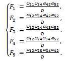
 . For demonstration purposes in Fig. 4a we present degree of the power as the weights of arcs of the digraph G, which along with the free electron and hole concentrations p and n, are incorporated into the probabilities of transitions. Eight trees grow into each vertex of this digraph [Fig.4a], so that total number of covering trees equals to 40. As mentioned in previous section, number of the trees can be found with help of the matrix K. However, we shall be interested only in the trees of largest weights in an asymptotical limit. Following a procedure for the search of the trees of maximal weight, e.g., by algorithm developed by Edmonds 4, one can find that there are only ten such trees [Fig. 4b]. By one maximal tree grows into each of the vertices 1, 2, and 3. Summing the weights of their arcs indicated in Fig. 4b, one can find that the weight of each of the trees is proportional to the 4th degree of the parameter of external excitation. Three maximal trees grow into the vertex 4 with weights proportional to the 3rd degree of the excitation parameter. Four maximal trees grow into the vertex 5 with weights proportional to the 2nd degree of the parameter of excitation. Therefore, in an asymptotical limit one can get: [1]=ω31ω23ω43ω54=
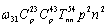 ,[2]=ω13ω32ω43ω54=
 , [3]=ω13ω23ω43ω54=
 , [4]=ω13ω54(ω23ω35+ω32ω24+ω23ω34)=
  (
( ω35+
ω35+ ω24+
ω24+ ), [5]=ω13(ω23ω43ω35+ω23ω34ω45+ ω32ω24ω45+ω23ω45ω35)=
 If the electro- neutrality condition p ≈ n is fulfilled, then the distribution function will depend on carrier density as follows:
 where
where 


 ω35)/Dwith the deno-minatorD=
 ). Analysis shows that upon increase of the injection level, occupation of the states 4 and 5 approaches zero inverse proportionally to n and n2, respectively. However, portions of defects in the states 1, 2 and 3 are stabilized on φ1, φ2 and φ3, accordingly. Incidentally we shall note that the transitions 4
 2 and 5
 3 are included in none of the maximal trees [Fig. 4b]. Therefore their elimination from the model does not affect noticeablyon the asymptotic limit of the distribution function. All the other transitions are used by the maximal trees. Therefore, even if probabilities of some of the transitions will be considerably smaller than ω42 and ω53, elimination of any of them may disturb the distribution function seriously. Thus, only after construction of maximal trees one can know whether influence of a transition on distribution function of the defects can be neglected or not.By using the distribution function one can find the rate of GR transitions. In the above example asymptotic limit of the rate of intra-center spontaneous transitions 3
 1, 4
1, 4 2 and 5
 3 will be equal to R31 = Ntotφ3ω31, R42 = Ntotφ4ω42/n and R53 = Ntotφ5ω53/n2. If any of these transitions are irradiative, then the rate of emission either saturates for the transition 3
 1, or decreases inverse proportionally to n for 4
 2 and to n2 for 5
 3. Section II of this paper discusses the technique of finding the stationary rate of GR transitions with help of the digraph of states.
3.4. Specular Features of the Models Described by Weakly Connected Digraphs
- So far we have considered the case when the digraph of states G is covered by the “growing into” type of trees. Namely in such case the distribution function can be found by the tree-weight rule described by Eqs.(12)-(15). Connected symmetric digraphs, strong digraphs, which are not necessarily to be symmetric, and the above mentioned examples described by symmetric digraphs possess the specific feature. A wider class of digraphs that has only one strongly connected component of sink-type, denoted further as the A-component, can also possess such a feature. Types of connectivity components are discussed in Appendix A. In this case all the vertices of the A-component (to be called hereafter as A-vertices and designated by iA) will be reachable from any vertex of the digraph G. Namely, all of them will be accessible mutually and also accessible from the other vertices which do not belong to the A-component (to be denoted by
 -vertices). They all will belong to the source and transit components. Because of this reason each A-vertex will be a root for at least one spanning tree and will, therefore, have a non-zero tree-weight. On the contrary,
  -vertices, being inaccessible from A-vertices, cannot be roots for spanning trees and, hence, their weights equal to zero. It is evident that at any initial distribution ofdefects on their states, occupation of the
  -states can steadily decrease, because probability of transition of the defects into the
  -states is equal to zero, while that going out from these states is not zero. So, more and more defects will gradually be accumulated in the A-states, since they are incapable of leaving the states into
  -vertices. In steady state conditions all the defects will occupy only A-states, whereas the
  -states will become completely unoccupied and transitions linking them with each other or with the A-states will be completely stopped. In view of ‘dying away’ of the
  -states during relaxation of the system into the steady state, at calculation of the stationary distribution function one can consider only the A-states and transitions, linking them. Then instead of the Eq. (15) one can use the following equation for the A- and
  -states, respectively.
 | (26) |
 | (27) |
 ) and not for the whole digraph G. Weight of the whole A-component in the denominator of the Eq.(26) is the sum of the tree-weights of all vertices included into it:
 | (28) |
 , two transit components
 and
and , and one sink component
 . Weights of the states not included into the A-component are equal to zero. It means that at the steady state conditions all the defects will be in the states 3, 4, 5, and 9. To calculate the tree-weights of the states one should sum up the weights of the trees covering the A-component [Fig. 5c]:
  =
= =ω5,4ω9,4ω4,3,
  =
= +
+ =ω5,4ω9,4ω3,4+ω5,4ω3,9ω9,4,
  =
= +
+ =ω3,4ω9,4ω4,5+ω3,9ω9,4ω4,5,
  =
= =ω5,4ω4,3ω3,9. According to the tree-weight rule [Eqs. (26)-(28)], the stationary distribution functions will be F3 = ω5,4ω9,4ω4,3/D, F4 = ω5,4ω9,4(ω3,4 + ω3,9)/D, F5 = ω4,5ω9,4(ω3,4 + ω3,9)/D, F9= ω5,4ω4,3ω3,9/D, F1,2,6,7,8,10,11 = 0. Here the denominator D is equal to the sum of the numerators of all the fractions. Note that, as the digraph G has the only A-component, one could also perform the calculation using the Eqs. (14) and (15), but then one had to deal with all 1368 (!) trees covering G and, after simplification of the fraction [Eq.(15)], one can get the same result. Therefore, the preliminary demarcation of the A-component in the digraph of states G may assist greatly in finding the distribution function Fi. This is one of the advantages of the graph theory over the other ways of deriving Fi by solving the system of equations.
 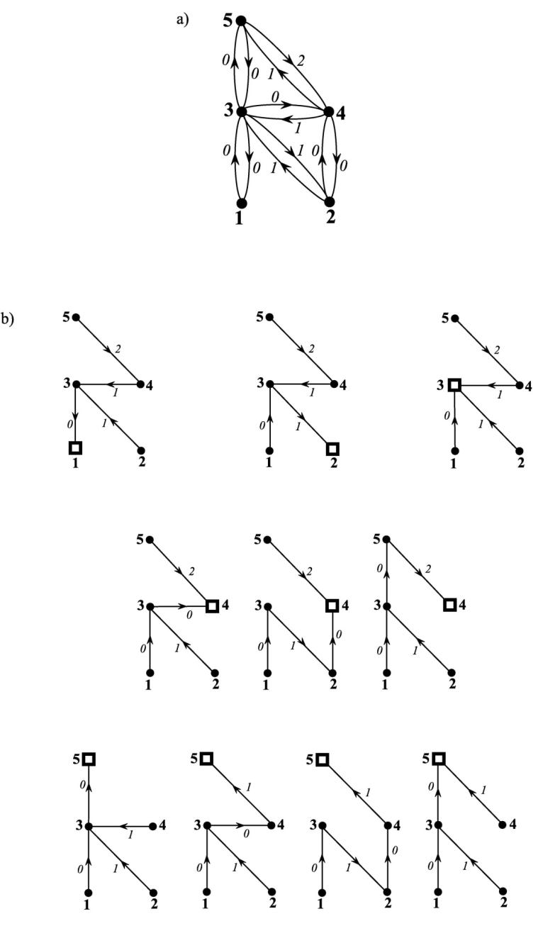 | Figure 4. (a) A digraph of states for a hypothetical defect with two-charge states with a ground state 1 and two excited states 3 and 5 corresponding to the empty defect, and a ground state 2 and excited state 4 corresponding to the defect with one trapped electron. Weights of the arcs of the digraph G are shown as the degree of the power, which along with the free electron and hole concentrations p and n, are incorporated into the probabilities of transitions. Eight trees grow into each vertex of this digraph, so that total number of covering trees equals to 40. (b) The ten rooted trees with the largest weight and determining the asymptotic values of the tree-weights of all the vertices. Exponent for the weights of the trees can be calculated by summing up the indicated weights of their arcs |
 and R2=[4,7], one transit component
 and two sink components A1 =[4,7] and
 If initially all the defects were in the states belonging, say, to the components T and R2, then after the steady conditions reached, all of them, evidently, will occupy the states of the A2-component, i.e. in the states 9 and 10. However, if initially some part of the defects were in the R1-component, then upon relaxing to the stationary state some defects will be locked in the A1-component, i.e. the defects will stay in the 5th state, and remaining defects will be in the A2-component. By virtue of mutual inaccessibility between states belonging to different A-components and of the absence of direct influence of them on each other, the set of states breaks up into subsets (more precisely, into mA), which are isolated each from other. The defects incorporated into each of the subsets will evolve according to internal regulations of the subset. By considering each subsystem corresponding to the A-component irrespective of others, we can conclude that the stationary distribution of defects within the A-component should obey to the rule described by the Eq. (26). Consequently, if the steady state is already reached and the portion of the defects incorporated into the first A-componentforms
 , into the second A-component forms
 , …, into the mA-th component forms
 , then the distribution function can be calculated by:
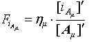 | (29) |
 | (30) |
 incorporated into the component Aμ (μ=1,…,mA) are determined by prehistory of reaching the stationary state and obey the natural requirement
 | (31) |
 shows that it is the sum of the weights of the trees covering only Aμ-component of the digraph G. Weight of the component is the sum of the weights of the vertices coming into it:
 | (32) |
 . By definition weight of a trivial tree consisting of only one vertex, is equal to unity. Tree-weights of both vertices in A2 are:
  =
=  = ω10,9 and
  . If as a result of the transient processes the portion of the defects in A1equals to
 , then their portion
  in A2 will be equal to (1–
 ) and the defects will populate their states as follows: F5 =
 ,
, 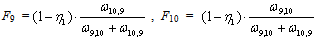 , F1-4,6-8 = 0. Again, as in the previous example, we have managed to obtain the distribution function easily due to the possibility of dealing only with the A-components of the digraph G.
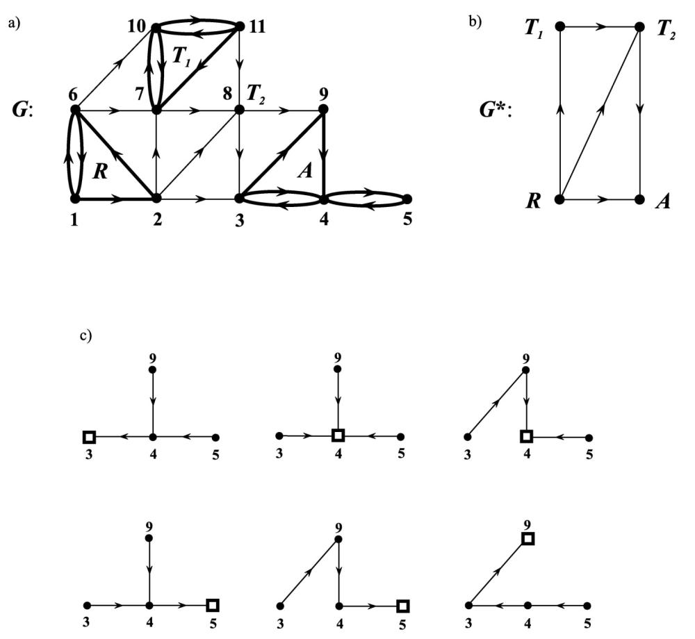 | Figure 5. (a) Weak digraph G with one source component , two transit components , two transit components  and and  and one sink component and one sink component . For visualization the strong components are depicted by bold lines. (b) Condensation of the digraph G* schematically illustrates the connections between the components. The step-by-step outflow of defects from R- and T1,2-states results in occupation of only the A-states 3,4,5,9 by the defects at steady state conditions. (c) The tree-weight of each vertex belonging to the A-component is determined by the trees covering the component. . For visualization the strong components are depicted by bold lines. (b) Condensation of the digraph G* schematically illustrates the connections between the components. The step-by-step outflow of defects from R- and T1,2-states results in occupation of only the A-states 3,4,5,9 by the defects at steady state conditions. (c) The tree-weight of each vertex belonging to the A-component is determined by the trees covering the component. |
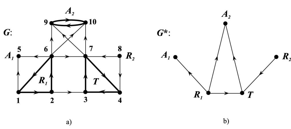 | Figure 6. (a) Weak digraph G with two source components  and R2=[4,7], one transit component and R2=[4,7], one transit component  and two sink components A1 =[4,7] and and two sink components A1 =[4,7] and . (b) Links between the components. In stationary conditions all defects will be only in A-states. Although the distribution of defects between the components A1 and A2 will depend on previous history of reaching the steady state conditions, distribution of defects on states within each of the A-component is determined by only the tree-weights of the vertices of the corresponding A-component . (b) Links between the components. In stationary conditions all defects will be only in A-states. Although the distribution of defects between the components A1 and A2 will depend on previous history of reaching the steady state conditions, distribution of defects on states within each of the A-component is determined by only the tree-weights of the vertices of the corresponding A-component |
 determine the relative populations of the states only within the Aμ-components and are independent of how the system approaches the stationary state. Therefore, for finding the normalized distribution function for
  one needs to know
  (μ = 1, …, mA) for mA connected with Eq. (17) and determining the portions of defects from their total number being in each of the Aμ-components. This is the relation between the rank of the system of algebraic Eqs. (3) and (4) and one of the numerical characteristics of the digraph G, which is the number of its strong components mA of sink type:
 | (33) |
4. Generation-recombination Processes
4.1. Digraph of States and the Rate of Generation-recombination Transitions
4.1.1. Some Quantities Describing the GR-transitions
- As a rule, transition of a defect from one state into another can occur by different channels, characterized by probability and change of the number of free carriers in each of the allowed bands. Transition probability of a defect from the state i into the state j by the particular channel
 will be denoted by
 . Change of number of the free electrons and holes caused by the transition will be denoted by
  and
and , respectively. For example, for transitions in Fig.7,
  = –1 [Fig. 7 a, d, e, and f],
  =0 [Fig. 7, b and c],
  =0[Fig. 7, a],
  = 1[Fig. 7, b, c, e, and f],
  = +1[Fig. 7, d]. The net transition probability ωij of a defect i
 j is equal to the sum of the probabilities of transitions by all possible channels:
 | (34) |
 will give the portion of the transition occurring by the particular mechanism α. Since at each such transition of a defect i
 j number of free carriers in their “native” bands varies by
  and
and , then the number of electrons in the conduction and valence bands changes on average by
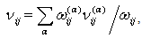 | (35) |
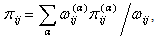 | (36) |
 and
and  characterizing separate mechanisms, thequantities νij and πij averaged over all the mechanisms will be non-integer. Let, for example, transition of an acceptor from the zero-charge state “0” into the negatively charged state “1” can occur by one of the three ways: (i) bycapturing an electron from the conduction band by the multi-phonon mechanism of energy dissipation. We shalldenote this channel by “a”. It is characterized by the probability
  , by
, by  and
and  . (ii) By the Auger mechanism with transmission of some energy to another free electron (termed as the channel “b”:
 ,
,  and
and  =0). (iii) By capturing an electron from the valence band termed as the channel “c”, described by the probability of generation of a hole
  and changes of the number of carriers by
  = 0 and
  = +1. Then according to Eqs. (34)-(36) each transition 0
 1 is accompanied by changes of the number of free electrons and holes
  =
= and
and  =
= , respectively. Here
 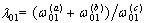 . In the limit
  , which means that the transition probability by the channel “c” is much smaller than that by the channels “a” and “b”, or, on the contrary, at
  , when the channel “c” is dominating, the magnitudes of
  and
and  will practically be coincident with those of
  and
and  corresponding to the dominating channel.Further, any transition i
 j is characterized by change of the number of electrons bound on a defect Δlij= lj– li, where li is the number of electrons on the defect in the i-th state. It is evident that Δlij is independent of the mechanism of the transition α, and it depends only on the initial i and final j states of the defect. Based on the fact that at any GR-transitions total number of carriers remains constant and the transitions only redistribute the carriers between the allowed bands and the defect one can write that
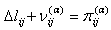 | (37) |
 | (38) |
 , then sum them up over all channels and divide them by the total transition probability ωij. Then, using the Eqs.(35) and (36) and accounting for the fact that Δlij is the same for all channels, one can get the Eq.(38).
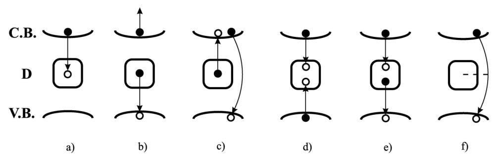 | Figure 7. Scripts of some transitions between the defect “D” levels and conduction/valence bands. The conduction and valence bands are marked as “C.B.” and “V.B.” respectively, and an electron and a hole are figured accordingly as the closed and open circles. (a) Capture of a conduction band electron by a defect, (b) recombination of an electron trapped on the defect with a valence band hole with transmission of some energy liberated to a free electron, (c) band-to-band recombination of an electron-hole pair with some part of energy spent for excitation of an electron from the defect to the conduction band, (d) simultaneous capture of one electron from the conduction band and another one from the valence band, (e) and (f) transitions consisting of simultaneous capture of a conduction band electron and a valence band hole (e) on the defect and (f) around the defect, that does not change number of electrons on the defect and, therefore, keeps its charge unchanged. Such a defect can nevertheless pass through the other quantum states |
4.1.2. Rate of GR-transitions at steady State
- The rate
 of the transitions of defects
  per unit volume is equal to product of density Ni of the defects in the i-th initial state by the probability of the transitions
 , i.e.
 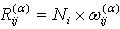 . Total rate Rij of transitions of defects i
 j, being the sum of all particular rates
 , is equal to product of the defect density Ni by total probability of the transition ωij: i.e.
  . Since each transition i
 j of the defect changes the number of free electrons on average by νij and that of holes by πij, then one can find the equation for the net rate of change of the number of free electrons Un and holes Up due to the defects
 | (39) |
 | (40) |
 | (41) |
 | (42) |
 ,
,  . Note that if
 , where γ and
  [L3T1] are the coefficients of the band-to-band recom-bination in the regular and distorted regions respectively, Vi is the volume of the region around the defect, then
  will give the additional probability of the band-to-band recombination to that in the absence of defects.In a stationary state both rates Un and Upare equal to each other, because predominance of one rate over the other would cause accumulation of one type of charge carriers, which is possible only at the non-stationary conditions. Proof of the assertion byEqs. (37), (39), and (40) is discussed in Appendix B. The quantity U ≡ Un= Up is the rate of GR-transitions, which we are interested in. It is equal to the stationary rate of decreasing the number of the free carriers in either of the allowed bands due to the defects. Commonly, U is calculated in two steps: firstly, the system of kinetic equations is constructed and then solved. It gives the stationary distribution function of defects on states Fi, and then U is found by the one of the Eqs. (39)-(42). Further we shall describe how the equation for the rate of GR-transitions can be constructed using the digraph of states of defects G and other possibilities of the graph theory in investigation of the GR processes through point defects.
4.1.3. Construction of the Equation for the rate of GR-transitions by Digraph of States
- In order to find the rate U directly from a digraph of states G one should first build up all functional digraphs (to be called hereafter as Φ-graphs)
 covering G. Φ-graph is a cycle C (loop is also permitted) and, perhaps, some trees will grow into the vertices of the cycle [1], which form a forest. An important feature of a Φ-graph is that exactly one arc outgoes from each of its vertex. If one of the arcs will be removed from the cycle C of a Φ-graph, then the Φ-graph will turn into a tree growing into the vertex, which the removed arc is issued from. On the other hand, if the root vertex of a “growing into” tree will be connected by an arc with some other vertex of the tree, then the arc will close a cycle and a Φ-graph will appear. Any Φ-graph can be constructed by this way. If a Φ-graph includes all vertices and arcs of a digraph G, then one can say that such Φ-graph covers G. Fig. 8 shows an example of a digraph G with a Φ-graph covering G that contain multiple arcs corresponding to competing mechanisms. The Φ-graph consists of the cycle C = 2
 5
5 6
6 2 and of the forest, containing two trees: T(2) = 1
 2 and T(6) = (7
 3)& (4
 3
3 6). Two Φ-graphs are considered as different, if their sets of arcs do not coincide. A digraph G may have several different Φ-graphs covering G. The subscript “k” at
  is used to distinguish such Φ-graphs. For example, the digraph G in Fig. 9a may be covered by fourteen Φ-graphs
  (k = 1,…,14) shown in Fig. 9b. Not all digraphs have Φ-graphs covering them, but any strong digraph includes at least one covering Φ-graph. Further we shall deal with the strong digraphs only, because in steady state conditions all defects occupy the states belonging to the strong (sink) components of a digraph of states G. The defects populating any A-component can be studied independently from others. Weight[
 ] of a Ф-graph
  is defined as the product of weights of all its arcs:
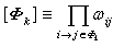 | (43) |
 . Expected change of number of electrons in the conduction band and holes in the valence band occurring as a result of single passing of a defect along the cycle Ck we shall designate accordingly by νk and πk:
 | (44) |
 | (45) |
 ] of all Ф-graphs covering a digraph of states G, magnitudes of νk for the appropriate cycles Ck, and also the tree-weights[i] of all the M-vertices of the digraph G, one can find the rate of GR-transitions by
 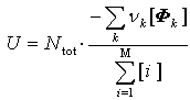 | (46) |
 , for which the quantity νk is not equal to zero. For the Ф-graphs the cycle Ck assigns to the defect such a closed path, along which the number of free carriers averaged over the great number of passages varies. Sign of the contribution depends on whether the free carriers will be generated (νk>0) or removed (νk<0) when the defect passes along the cycle Ck. For νk>0 (νk<0), the contribution is negative (positive) in accordance with the above-mentioned convention on the sign of electronic transitions rate. The Ф-graphs with a cyclic path Ck, along which number of the free carriers does not vary (i.e. νk = πk= 0), do not make the contribution to the rate U.
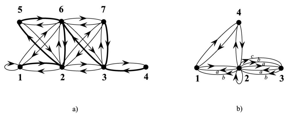 | Figure 8. (a) Digraph G with one of its Φ-graphs. The arcs not included into this Φ-graph are plotted by dots. (b) An example of a digraph of states G with multiple arcs corresponding to the different mechanisms of the defect transitions |
 and
and  denote a Ф-graph and its cycle. Arcs of the cyclecorrespond to separate channels of transitions and accordingto the above definition, weight of the Ф-graph[
 ] will be equal to product of weights of all its arcs. Furthermore, it will be convenient to combine addends in the numerator in
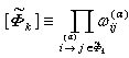 | (47) |
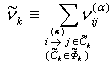 | (48) |
 is total change of number of conduction band electrons due to transitions of the defect along the cycle
  by the mechanisms, appropriate to this cycle. So, using the above definitions one can rewrite the Eq.(46) as:
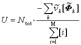 | (49) |
 covering G can be divided into a few groups. In each of the groups all the Ф-graphs have the cycles
  passing the same vertices in the same direction, but only via different multiple arcs. It is convenient to use the notation
 . Here the subscript k points to the group, and the superscript μ shows the numbers the cycles within the k-th group. It is evident that the same set of different forests will grow into any μ-th cycle of the same group k, and we shall designate this set of forests by
 . The forests are considered to bedifferent, if composition of trees is different each from other. We shall define the total weight[
 ] of all set of forests as sum of weights of each concrete forest, and that of a single forest as a product of weights of all its trees, i.e. in fact as a product of weights of all arcs comprising thisforest. Then it is possible to present Uas
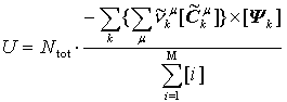 | (50) |
 is the total (integer) change of number of free electrons caused by transitions of defects along the cycle
 . Weight[
 ] of the cycle is equal to product of weights of its arcs. Let us also note that if there are no trees grown into the cycles
  of the k-th group, then theweight[
 ] should be formally put equal to unity.To clarify the above definitions let us consider the digraph G in Fig.8b, which contains 14 cycles bunched in seven groups: first group includes two cycles
 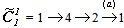 and
and 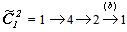 , passing the vertices 1,4,2, and 1 in this order and is distinguished by the multiple arcs
 and
and . Second group consists of one cycle
 . Third group includes two cycles
 and
and 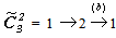 . Fourth and fifth ones contain by one cycle
 and
and respectively. 6thgroup includes six cycles

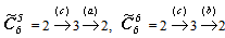 and, finally, seventh group is the loop
  Two variants of forests grow into each of the two cycles of the first group: one forest consists of the tree
  and another one consists of the tree
 . The same concerns to the cycle of the second group, so we can write
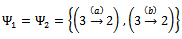 . Four types of forests grow into the cycles of the third group:
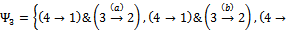
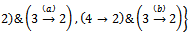 . Six variants of forests grow into the cycle
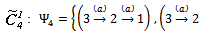
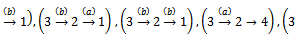
 and four forests grow into the cycle
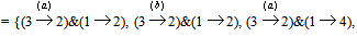
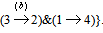 Three variants of forests grow into the cycles of the sixth group:
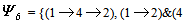
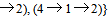 and, at last, six variants of forests grow into the sole vertex of the loop
 . Each of them is a tree covering the digraph G:
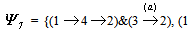
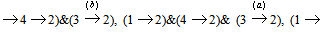
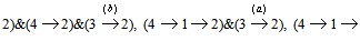
 . Any of the forty eight Ф-graphs
  (k = 1,…,48) covering G is constructed by conjunction of one of these cycles with one of these forests growing into the chosen cycle. Hence, the numerator of Eq. (50) will contain 48 addends. Among them there will, for instance, be such ones: {


 . Note that the weight[
 ] coincides with the tree-weight of the 2nd vertex [2], and this is a general rule that if
  is a set of forests growing into the vertex i of a loop i
 i, then the weight[
 ] will give the tree-weight[i] of this vertex.In a non-degenerate case it is possible to make further progress, if in a model reverse transition is also taken into account together with each allowed transition. As shown in Appendix D, in this case the equation (50) becomes
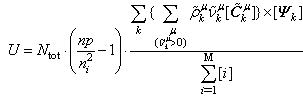 | (51) |
 are taken into account which
  and the following notation is used:
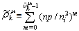 | (52) |
 is present in the equation for the rate U. Since the rest fraction is positive, one can conclude that at high injection levels
 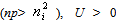 , i.e. the rate of recombination will exceed the rate of generative transitions. Upon exclusion of the charge carriers
 . Then the defects will play a role of centers for free carrier generation. At equilibrium state product of the free carrier densities (np)eq is equal to
  and the rate of GR-transitions Ueqequals to zero in complete agreement with the principle of detailed balance. Note that the equality Ueq = 0 can also be derived from the general Eq. (46) or from its variants Eqs. (49) and (50) which, distinct from the Eq.(51), holds true in the degenerated case (Appendix E).It should be noted that the Eq. (51) is universal for all models of recombination through point defects. As we have tested, the equations for the rate of GR processes derived so far for particular models developed, e.g., by Shockley and Read30, Hall31 for single level stable defects, by Evstropov34for recombination through excitons, by Karageorgy-Alkalaev, et. al. for donor-acceptor pairs39 and hypothetic model of metastable defects42, by Kanaki et. al. for bistable defects26etc., are particular cases of the Eq. (51). Also, we note that the Eq. (51) has been derived without designing the system of kinetic equations. Preliminary knowledge on distribution of defects on states or derivation of it through mathematical manipulations was not needed. Analysis of Eq. (51) shows that the rate U contains the terms
 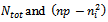 . Consequently, dependence of charge carrier lifetime on concentration of recombination centre
  as well as the approximation
  are universal for all types of the centers from point defects.
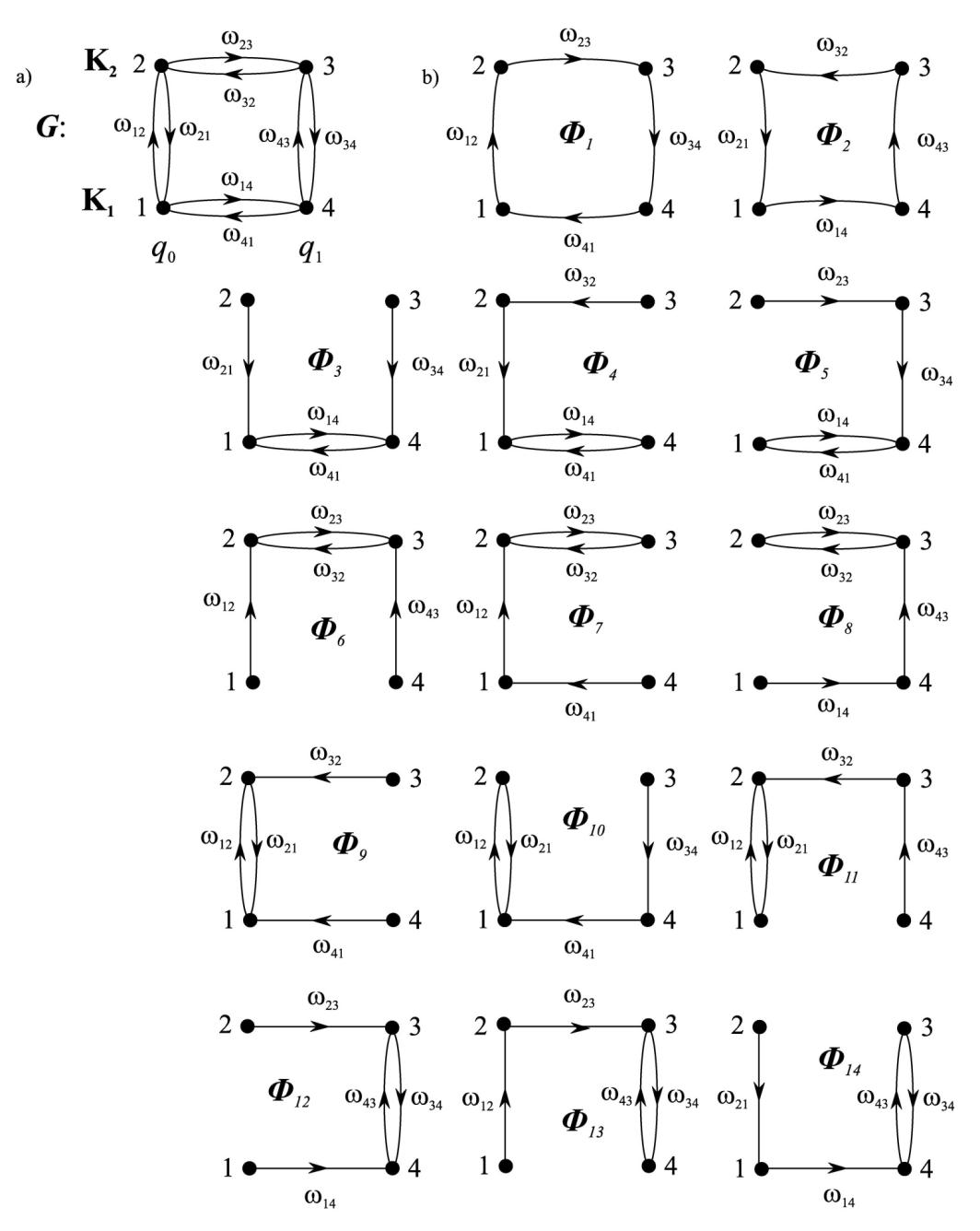 | Figure 9. (a) Digraph of states G corresponding to a bistable defect, which can be either of its two-charge states with two ground states 1 and 4 and two excited states 2 and 3. Space configurations Q1 and Q2 correspond to the ground and excited states, respectively. In the states 1 and 2 the defect is ‘empty’ and is in the charge state q0. In the states 3 and 4 the defect has one captured electron and its charge is q1 = q0 – 1. (b) all Φ-graphs  (k = 1,…,14) covering G. Weights of the Φ-graphs determine the rate of GR-transitions U (k = 1,…,14) covering G. Weights of the Φ-graphs determine the rate of GR-transitions U |
4.2. Application of the Results to Particular Models of Generation-recombination Processes
4.2.1. Astatic and Static Involvement of Defects in Generation-recombination Processes
- By analysis of charge carrier GR we came to conclusion that participation of defects in these processes can be characterized as “astatic” and “static”. It can be said as static if as a result of recombination there is no change of charge state of the defect. Otherwise it can be considered as astatic. Fig. 7 (a)-(f) shows some examples of astatic and static involvements of a defect in charge carrier recombination. In Fig. 7(a)-(d) we display the examples of astatic involvement, which include: capture of a conduction band electron by a defect[Fig. 7a], recombination of the trapped electron with a hole accompanied by transferring the energy to a free electron[Fig. 7b], band-band recombination of an electron-hole pair with some part of energy spent for excitation of an electron from the defect to the conduction band[Fig. 7c], simultaneous capture of one electron from the conduction band and another electron from the valence band[Fig. 7d]. These transitions are accompanied by recharging the defect by losing one electron[Fig. 7 (b), (c)], gaining one electron[Fig. 7 (a)] and[Fig. 7 (d)] two electrons. So, they can be called as astatic participation of the defect in the processes of generation and recombination. The processes can be accompanied by intra-center Auger transitions 22 (not shown in the figures). The examples of static involvement of defects in charge carrier recombination are shown in Figs. 7 (e) and (f). The transition in Fig. 7(e) consists of capture of an electron from the conduction band and a hole from the valence band by the defect at the same time and this process does not change number of electrons at the defect andits charge state. However, the defect can nevertheless be passed into some other quantum state, if, e.g., an electron and a hole will be trapped into different electronic orbitals. In the latter case the defect “invisibly”, i.e. without any apparent consequences for itself, participates in the transition, providing an extra channel of recombination for electrons and holes. It should be emphasized that nature of this process is completely different from the one-electron mechanism of recombination when a defect captures a carrier of one type and only after that it captures another type of charge carrier. In our case we deal with capture of both types of charge carriers simultaneously. Note that the mechanism can result in discrepancy between the experimental data and the recombination rate calculated within the band-to-band recombination without including the defects into account. However, involvement of defects could be testified, for example, by radiation, which may accompany the transition, because it will differ from a mere band-to-band radiation, and also presence of dependence of band-to-band recombination rate on the density of defects. Also, it can be testified by difference of calculated and experimentally determined carrier lifetimes. Similar to processes in Fig. 7(e), those in Fig. 7(f) do not cause recharging the defect. Distinct from the band-to-band recombination in the regular lattice, it is subjected to influence of the nearby defect [Fig 7 (f), dotted line]. This influence can be, e.g., the result of transmission to the defect part of the energy liberated during carrier capture and of the momentum, initiating thus the intra-center transformation (not shown in the Fig.7). The intra-center transformation can be the transition between different states of atomic multiplets or different space configurations of atoms. Also, the defects can influence a course of the band-band recombination indirectly without making any transitions at all. Indeed, any defect always distorts more or less vast region of the lattice, whereas the probability of the band-to-band recombination depends on the lattice. In regular lattice it can differ significantly from that in distorted one. If the volume of the distorted region around each defect is V0, then in the unit volume of the crystal the distorted volume should be NDV0, where ND is a density of defects. So, if γ and
 [L3T1] are the probabilities of the band-band recombination rates γnp and
  np in undistorted and distorted lattice regions, respectively, then the average recombination rate per unit volume will be characterized by the effective constant γeff = γ×[1 – NDV0] +
 ×NDV0 , which exceeds γ by ~10% at ND = 1018 cm3, V0 ~ 1020cm3 and
  = 10. Both examples in Figs.7 (e) and (f) display that influence of defects on a course of GR-transitions cannot, necessarily be accompanied by transitions of defects between their states, but also be (e) latent and (f) passive, be involved in the GR processes without changing their charge state. That is why involvement of defects in such processes could naturally be termed as “static” in contrast to those (a-d) termed as “astatic”.
4.2.2. Rate of Static Mechanism of Recombination
- Note that the defect in the i-th state can influence on the rate of electronic transitions in the system, without changing its charge state. On digraph of states G it is pointed out with a loop incident to the i-th vertex. This is quite natural: a loop, as well as any arc on a digraph of states, indicates some transition in the system with involvement of the defect, but such transition does not take the defect out of its state. Then the above equations for the rate of GR-transitions U may be split up into two terms Uast and Ust:
 | (53) |
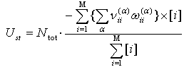 | (54) |
 ] of a loop
  is the weight
  of its sole arc
 , and the total weight[
 ] of all forests growing into the sole vertex i, gives the tree-weight[i] of this vertex. Here we will discuss the following important question as to when the static mechanisms of influence of defects on GR processes should be taken into account along with the astatic ones. Suppose that the recombination theoryforadefect without static effects has already been developed. It can be, e.g., the theory developed by Shockley and Read30, and Hall31describing the single ionized defects without excited states. Digraph of states G, corresponding to such defects has no loops in it. To account for the static mechanisms, one should add loops into the digraph G. As mentioned earlier, the static mechanism does not take the defects out of their charge states, but influences on distribution function of the defects on their states and the rate of GR-transitions indirectly through variations of free charge carrier concentration. One could also come to this conclusion from the diagram point of view. Indeed, presence or absence of loops in G has no effect on tree-weights [i] of vertices of G, since the loops are not the part of the trees covering G. Hence, the distribution function Fi which equals to the ratio of the tree-weight[i] to the total tree-weight [G] of the digraph G [Eqs.(39)-(40)] remains unaffected by the loops. Presence of loops influences only on the second addend in Eq.(53), i.e. on the static GR-transitions rate Ust, without affecting Uast. Based on the above-discussions one can say that static effects may be taken into consideration at any stage of developing the statistical theory of GR processes, since they can be studied irrespective of the static ones. Therefore, the recombination theory which does not include the static effects is not useless, because it provides us with the term Uast in Eq.(53). If a defect has a noticeable static influence, then it will be enough first to calculate the rate of the static GR-transitions Ust using, e.g., the usual function of distribution of such defects known from SRH theory [Eq. (54)]. Then one should add the result to the astatic GR rate Uast obtained within the framework of the above theory.
 4.2.3. Examples of Constructing the Equation for the rate of GR-transitions by a Digraph of States
- As the first example we shall consider a defect with M-charge [Fig. 10], but without excited states described by a digraph of states G [Fig.10a]. i-th vertex (i = 1,…,M) of the digraph corresponds to the defect with (i–1) captured electrons. So the 1st vertex corresponds to the “empty” defect with a charge q0, the 2nd vertex corresponds to the defect with one captured electron and with a charge q1= q0 – 1, etc. There are (M–1) Ф-graphs
 (k = 1,…,M–1) covering G. As it is seen from Fig. 10b, the Ф-graph
  consists of a cycle Ck= k
 (k+1)
(k+1)  k given by a couple of counter arcs linking the adjacent vertices k and (k+1), and also of the trees 1
 2
2 …
… (k–1)
(k–1)  k and M
 (M–1)
(M–1)  …
… (k+2)
(k+2)  (k+1) growing into the vertex k and (k+1) respectively. The terminal vertices 1 and M may be formally considered as roots of the trivial trees made up of only one vertex and have no arcs. Weight of such trees is assumed to be equal to unity. According to the Eq. (43), to find the weight of the Ф-graph one should multiply the weights of all of its arcs:
 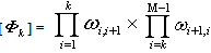 | (55) |
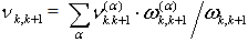 | (56) |
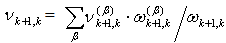 | (57) |
 | (58) |
 2
2 …
… (i–1)
(i–1)  i
i (i+1)
(i+1)  …
… (M–1)
(M–1)  M grows into the i-th vertex of the digraph G. It determines the tree-weight:
 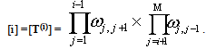 | (59) |
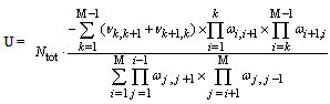 | (60) |
 | (61) |
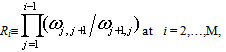 | (62) |
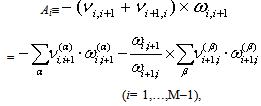 | (63) |
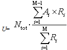 | (64) |
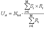 | (65) |
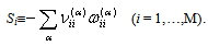 | (66) |
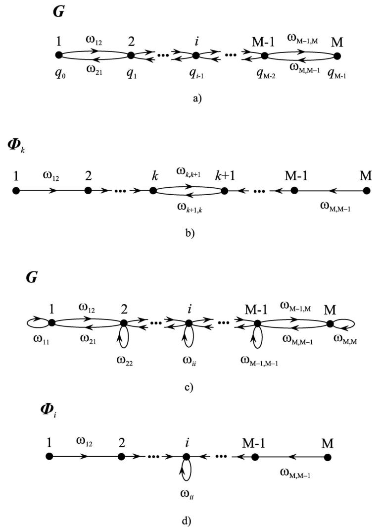 | Figure 10. (a) M-vertex digraph of states G for M-charge defect without excited states. Absence of loops indicates that the static effects are neglected. (b) One of the (M–1) Φ-graphs  (k = 1,…,M–1) covering the digraph G. (c) Digraph of states G of a defect of the above type, which accounts for bothtypes of transitions with astatic and static influence. (d) Digraph G containing Φ-graphs (k = 1,…,M–1) covering the digraph G. (c) Digraph of states G of a defect of the above type, which accounts for bothtypes of transitions with astatic and static influence. (d) Digraph G containing Φ-graphs  with the loops along with the Φ-graphs with the loops along with the Φ-graphs  . . |
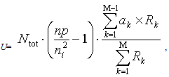 | (67) |
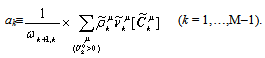 | (68) |
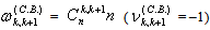 | (69) |
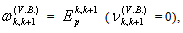 | (70) |
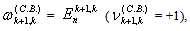 | (71) |
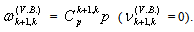 | (72) |


 Here
Here  and
and  on the arrows indicate the band, which interchanges by carriers with the defect level. Let us now calculate total change of the number of conduction band electrons along each of the cycles:
 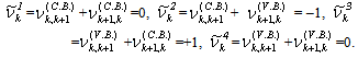 | (73) |
 gives positive
  and, consequently, it is the only cycle that should be taken into account at calculation of the coefficients ak in Eq.(68). Weight of the cycle is
 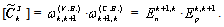 | (74) |
 , calculated by Eq. (52), is equal to unity. Thus, the coefficients ak become
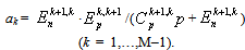 | (75) |
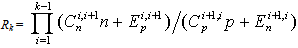 | (76) |
 2 and 3
 4 keep the charge of the defect constant and correspond to its transformation, whilst the transitions 1
 4 and 2
 3 are accompanied with recharging of the defect without changing its space configuration. The transitions 1
 3 and 2
 4, corresponding to recharging of the defect simultaneously with configurational changes have not been included into the model. Theory of recombination through such defects was studied, in particular, in Ref. 26, 41 within the kinetic approach 41 and graph theory 26. Furthermore, in previous chapter distribution function has been derived using the digraph of states G:
 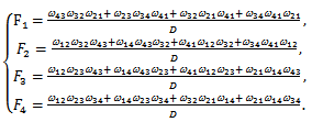 | (77) |
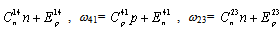 , ω32=
 . Probabilities of configurational transitions ω12, ω21, ω34 and ω43 will be determined by the mechanisms of passing of components of the defect between different positions in a crystal lattice. Also, we assume that free carriers do not participate in these transitions. In this case the latter probabilities will be independent on n and p.The digraph under consideration has 14 Ф-graphs
  (k = 1,…,14) shown in Fig. 9b. The Ф-graph
  contains the cycle C1 = 1
 2
2 3
3 4
4 1,
1,  includes the C2 = 1
 4
4 3
3 2
2 1,
1,  contains of C3 = 1
 4
4 1,
1,  contains C4 = 2
 3
3 2,
2,  contains C5 = 1
 2
2 1 and
1 and  contains C6 = 3
 4
4 3. In a non-degenerate case, one can derive the equation for Ufrom the Eq.(51). The cycle C1 can be passed by four ways distinguished each from other by mechanisms of transitions along the path
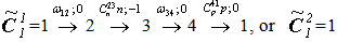
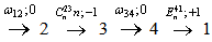 or
or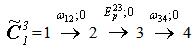
 , or, at last,
 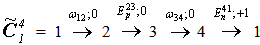 . The two parameters located above the arrows correspond to the probability
  of transition by the channel α and to the change of the number of conduction band electrons
 . Let us now count up the total changes of the number of free electrons for these cycles:
  = 0 – 1 + 0 + 0 = –1,
  = 0 – 1 + 0 + 1 = 0,
  = 0 + 0 + 0 + 0 = 0 and
  = 0 + 0 + 0 + 1 = 1. Among all of these cycles the only cycle
  has the positive
 , so we need the weight of only this cycle[
 ] = ω12
 ω34
ω34 and the sum in Eq.(52) equals
  . We shall now consider the next cycle C2. It can also be passed by four ways:
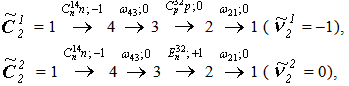
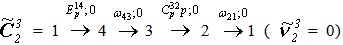 and
and 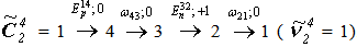 . Among the ways only
  is of interest:
 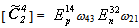 and
and . One can see from Fig. 9b that there are no trees grown into the cycles C1 and C2 except the trivial ones. According to the remark to the Eq. (50), weights of the forests[
 ] and[
 ], included into the Eq.(51), are equal to unity. Further, there are the following ways to pass the cycles C3 and C4:
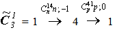
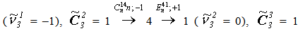
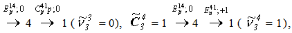
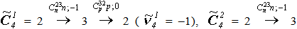
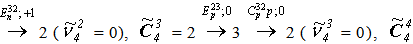
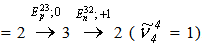 . Among them only two ways havepositive increments of the number of free electrons with weights[
 ] =
] =  and[
and[ ] =
] = . Sums in Eq.(52) for the weights are equal to unity:
  . Three versions of forests grow into the cycle C3: one of them consists of two trees (2
 1) and (3
 4). The forest together with the cycle C3 produce the Ф-graph
 . Second one is the sole tree (3
 2
2 1), which is well seen from
 . Third one is the tree (2
 3
3 4) (see
 ). Totalweight of all these forests is[
 ] = ω21ω34 + ω32ω21 + ω23ω34. Three different forests also grow into the cycle C4: one of them includes two trees (1
 2) and (4
 3). Another one includes the tree (4
 1
1 2) and the last one is the tree(1
 4
4 3), so that[
 ]=ω12ω43 +ω41ω12 +ω14ω43. Finally, both cycles C5 and C6 consist of the intra-center transitions 1
 2 and 3
 4, which do not change numbersof free electrons (ν12= ν21= 0 and ν34= ν43= 0). Hence, theФ-graphs
  which contain these cycles do not make a contribution into the rate U. Now we should substitute these results into the Eq. (51), which yields the equation for therate of astatic GR-transitions via the given defects:
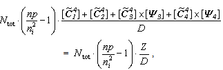 | (78) |
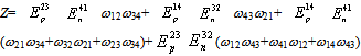 | (79) |
4.2.4. Inertial Properties of An Ensemble of Defects at High Injection Levels
- In this section we shall consider the question related to influence of defects on the rate of GR-transitions at high levels of injection of charge carriers. This leads to theproblem of finding asymptotical behaviour of U at large concentrations n and p, because lifetimes of the charge carriers and GR-currents in power devices depend on these parameters. Some defects are capable of providing highGR-transition rate at high injection levels. Such defects can be referred to as “inertialess”, meaning their capabilityto capture carriers of both signs without any time delay. Even if there is some time-lag then it drops fast with increasing the injection level. Some defects might showresistance or disinclination to GR processes. As a result they can provide only limited recombination rate, whichtends to some finite value (e.g., to zero) as the injection level increases. Such defects should be classified as “inertial”, since the defects will spend on more time in the recombination-passive state without capturing the injected carriers.It leads to lagging ofrecombination rate compared to increase of the number of injected carriers. There is also third type of defects with the rate of GR-transitions equal to zero at any levels of injection. These are, for example, the so-called sticking centers, exchanging by charge carriers with only one of the allowed bands. On the one hand inertial properties of an ensemble of defects will depend on the pumping condition. The Shockley-Read-Hall type recombination centers, e.g., might become inertial at single carrier injection as well, since U reaches its maximal value determined by concentration of charge carriers. On the other hand, inertial properties depend on the scheme of allowed transitions of defects, i.e. on the properties of a digraph of states G. In this section we shall derive those features of G that make the ensemble of defects inertial or inertialess, considering non-degenerate case and excluding the Auger processes from consideration. Here we shall formulate the criterion of lack of inertness, which is common for any types of defects.We shall ascertain the expected asymptotical behaviour of the GR-transition rate U in a non-degenerate system excluding the Auger processes from consideration. In these conditions probability of transitions of the defects by capturing the electrons from the allowed bands is ωij=
 . The rate of emission of an electron from the defects is
 . Probabilities of intra-center transitions are assumed to be independent of the free carrier concentrations. Concentrations of the injected carriers will further be termed as “the parameters of excitation” (abbreviated to “PE”). For pumping of only electrons(holes) PE is the concentration of only electrons n (holes p). For bipolar carrier injection the role of PE will play both n and p. Then it is seen that the probabilities of any transitions in the system at high levels of injection will be proportional to the 0th or 1st degree of PE: ωij∝ PE0 or ωij∝ PE1 (in another notation, degωij= 0 and degωij= 1). Under these circumstances for the inertialess defects the asymptotic dependence of U on the injection level cannot be other than linear, i.e. U∝ PE1. Indeed concentrations of defects Ni (i= 1,…,M) should tend to their constant asymptotic values as the injection level increases, so that
 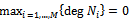 and, in virtue of Eq.(53),
  It should be noted here that this is the particular case of more general statement which says that if the maximal possible magnitude of the exponent (k) in the dependence of the transition probabilities ωij on PE is, say, kmax, then the exponent k in the asymptotic dependence U∝PEk may be varied up to kmax (it can be proven just as the above case). When kmax = 1, one can deal with the above case. So, the ensemble of defects to be considered as inertialess there must be probabilities with positive sign of the exponents. However, this requirement, which is usually fulfilled, is only the necessary one, but not sufficient yet. For non-degenerate system without Auger effects included into consideration one more necessary requirement of lack of inertness is active: carrier injection must be bipolar, otherwise the ensemble of defects will be inertial. This is a merely consequence of a more general statement that U may reach its maximal possible value of exponent k = kmax only at bipolar carrier injection. About inertial defects one can say they can lead to power dependence of the recombination rate U∝PEd. Here d is integer, which can be varied in the range:
 | (80) |
 | (81) |
 i1 with the probability
  proportional to PE1. Let us write down the equation for the defect density Ni through the tree-weights of vertices of the digraph of states G:
 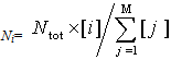 | (82) |
 , then the same proportionality[j] ∝
 will take place for the tree-weight of an appropriate state. tj coincides with number of arcs of the tree T(j) with weights proportional to PE1. Therefore, population of the state i will not become vanishing only if the vertex i is a root of at least one tree
  with maximal parameter
 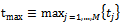 . Thus, for the ensemble of defects to be inertialess it is necessary and sufficient, that an arc
  of weight
  ∝ PE1 will be issued from the vertex i, which is a root of a tree of asymptotical weight[
 ] ∝
] ∝ . Then in the digraph G there will necessarily be such a tree, growing into the vertex i1 with weight proportional to
 . An arc will exist issued from the vertex i1with the weight proportional to PE1. If one removes an arc, e.g., i1
 i2from the tree
  and adds another one
  , then one can get a new tree
  growing into the vertex i1 with deg[
 ]=deg[
 ] + deg
 – deg
– deg = tmax+1–deg
 . Since the degree in the power
  of the weight of the tree
  cannot exceed the maximum value tmax and that the probability of any transition, including
  2 can be proportional to only PE0 or PE1, one comes with necessity to equalities deg[
 ] = tmax and deg
 = 1. For the same reasons it will turn out that the vertex i2 will be a root of at least one tree of maximal asymptotical weight proportional to
 . Also, an arc issued from this vertex with weight proportional to PE1. Following this way we can pick up a set of vertices i, i1, i2,…,iN of the digraph G, which are mutually connected with the arcs with weights proportional to PE1. Each of the vertices is a root of the trees with weights proportional to
 . Hence, one can conclude that the ensemble of defects can be said to be inertialess in the following cases:1) The digraph of states G has such a subset of vertices, which are mutually reachable with the arcs with weights proportional to PE1. Such a subset of vertices will further be referred as “non-inertial recombination component” (NIRC);2) The tree-weights of vertices in a NIRC must have the greatest possible growth rate, i.e. be proportional to
 . It is sufficient for the weight of at least one vertices of NIRC to have such an asymptotic limit, because the weights in asymptotical limit are proportional to each other. This note comes out from the following statement of the graph theory: if a group of vertices of a digraph G are connected by the arcs of equal and maximal weight in such a manner that all of them are mutually reachable, then the heaviest trees covering G and growing into these vertices will be of equal weight and, therefore, will contribute equally to the tree-weights of the vertices.Both signatures of lack of inertness of recombination properties can easily be tested for any complicated scheme of allowed transitions of defects. Before discussing the inertial properties of defects within the framework of the graph theory, we would like to specify their physical meaning.As it is clear from definition, a NIRC is such a group of defect states, which by capturing a free electron(hole) can be immediately ready to capture a hole(electron). Depending on features of the scheme of allowed transitions and of injection conditions the digraph of the defect states G may have one or more NIRC’s, or no NIRC at all. In case of single polar injection presence of NIRC becomes impossible. For a defect to be able to make a cyclic passage within a NIRC by capturing the injected carriers, it should capture the same number of electrons and holes, which implies bipolar injection. So, being in any non-inertial state a defect turns out to be able to capture any type of free carrier, and probability of such captures will increase with increasing PE. A question arises as to what happens if a defect abandons the NIRC? There are two possibilities. One of them is the defect can immediately or during the time of order PE-1 passes into another NIRC, and will again be recombination-active. It can also pass into another state and be unable to capture the injected carriers. Such states are termed as “recombination-passive” (RP). The defect can quite the RP-state due to transition with probability proportional to PE0, intra-center transition, transition accompanied with generation of a free carrier, but not capture, or single polar injection. A defect being in a certain RP-state can be out of the recombination activity for some time at any level of injection. Such defects will hamper the rate of GR-processes. Therefore, for an ensemble of defects to be non-inertial the scheme of allowed transitions must have at least one NIRC, i.e. such groups of defect states, which have no impediments for carrier recombination. This is the first repoint related to lack of inertness of defects. The other possibility is that the average time to be spent by a defect in the NIRC’s, i.e. the lifetimes of the NIRC-states, should not tend to zero with increasing the injection level. Otherwise number of the recombination active defect states will vanish with increasing the number of free carriers. It is in favour of population of RP-states resulting in inhibition of recombination. This is the second point of the above condition. Note that here we have used implicitly the ergodic properties of the steady state. The relative portion of time, which a defect spends in such a quantum state, coincides with that for all defects of the ensemble, which occupy the state at any time.As an example we shall construct asymptotic equation for the recombination rate through the donor-acceptor pairs (DA-pairs). In the simplest case the DA-pair can be in four different states:[D+A0],[D0A0],[D+A–] and[D0A–] [Fig.11], which are associated with the vertices 1, 2, 3, and 4 of the digraph G in Fig.11a. In an “empty” state[D+A0] the donor level is ionized, and the acceptor is neutral, so a charge of the pair is q0= +1. In the states [D0A0] and [D+A–] one captured electron is located in the donor or in the acceptor level, respectively. Therefore in both of the states the pair is electrically neutral: q1= 0. In the state[D0A–] the donor is neutral, and the acceptor is ionized. So the charge is q2 = –1. The transition 1
 2 is capture of an electron from an allowed band which will be localized on the donor. Probability of thisprocess is
  . One can get
  for the reverse transition, ω13 =
  forthe electron-capture from an allowed band into the acceptor, and ω31=
 for the reverse process. Probabilities of the remaining transitions are ω24 =
 , ω42 =
 , ω34 =
 , ω43 =
 . Probabilities of intra-center transitions ω23 and ω32do not dependon free carrier concentrations. According to Eq.(54) the rate of GR-transitions through such defects is given by the equation
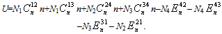 | (83) |
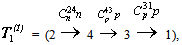 | (84) |
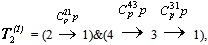 | (85) |
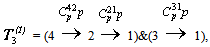 | (86) |
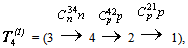 | (87) |
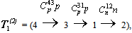 | (88) |
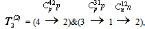 | (89) |
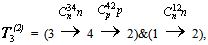 | (90) |
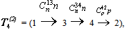 | (91) |
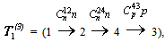 | (92) |
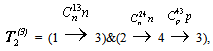 | (93) |
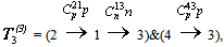 | (94) |
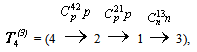 | (95) |
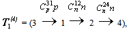 | (96) |
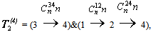 | (97) |
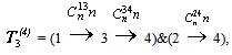 | (98) |
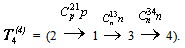 | (99) |
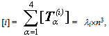 | (100) |
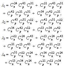 | (101) |
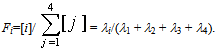 | (102) |
 | (103) |
 | (104) |
 2 and 2
 1, as well as 3
 4 and 4
 3 due to exchange by an electron only with the conduction band but not with the valence band? So, probabilities of the transitions are: ω12 =
 , ω21 =
 , ω34=
 and ω43=
 . The digraph G contains now two NIRC’s: one of them includes thevertices 1 and 3, which are mutually reachable due to the transitions
  and
and  , another NIRC holds the vertices 2 and 4, coupled by transitions
  and
and  . The asymptotic tree-weights of the 2nd and 4th vertices are determined by the following trees respectively:
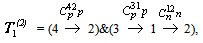 | (105) |
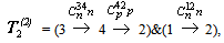 | (106) |
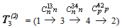 | (107) |
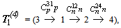 | (108) |
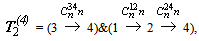 | (109) |
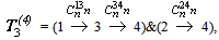 | (110) |


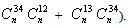 The trees growing into the 1st and 3rd vertices contain not more than two arcs with weights proportional to PE1, therefore, [1] ∝n2 and[3] ∝n2. Thus, at high levels of injection the defects will occupy only the 2nd and 4th states:
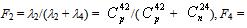
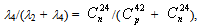 whereas thepopulation of the 1st and 3rd states will decrease in inverse proportion to n. Presence of the ever populated NIRC provides the ensemble of such defects to be non-inertial:
 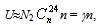 | (111) |
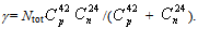 | (112) |
 occur only by electronic exchange with the valence band, but not with the conduction band, so that ω24 =
  and ω42 =
 . Corresponding digraph of states G in Fig.11c has one NIRC with the vertices 1 and 3. The state[D0A0], which the 2nd vertex corresponds to, is the recombination-passive one, since the defect being in this state cannot capture the injected carriers. Asymptotic magnitude of the tree-weight of the 2nd vertex is determined by the trees
 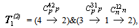 | (113) |
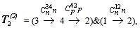 | (114) |
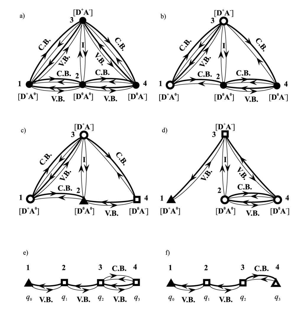 | Figure 11. (a) to (d) are the digraphs of states G for a donor-acceptor pair[DA] which can be in four different states. The bipolar injection is supposed. All these models differ by their sets of allowed transitions. A pair of counter arcs marked as “C.B.” means the possibility of recharge of the defect due to electronic exchange with the conduction band. The one marked as “V.B.” means the transitions with carrier exchange with the valence band. The letter “I” denotes intra-center transitions. Arcs corresponding to capture of charge carriers and having, therefore, the weights proportional to PE1, are shown as the bold arrows. Circles show the vertices, which come into some NIRC. The delta circuits are the vertices corresponding to the recombination-passive states. In such states the defect cannot capture the injected carriers. All the remaining states are marked by squares. The solid vertices correspond to the states, whose population does not vanish with increasing the injection level. The remaining states, which become empty in an asymptotical limit, are pictured as empty. (e), (f) The digraphs of states G for four-charge defect without excited states for (e) the hole and (f) bipolar injection |
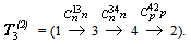 | (115) |
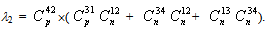 The trees with maximal weights proportional to n2 grow into the remaining vertices: for i = 1,3 and 4[i] = λin2, where
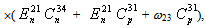

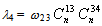
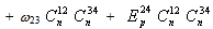
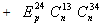
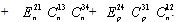 Therefore, in asymptotic limit all defects will be accumulated in the RP-state
  , whereas population of the rest states decreases according to
 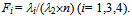 | (116) |
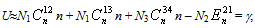 | (117) |
 . Such a saturation of the rate U results in linear increase of carrier lifetimes with increasing the injection level: τn≈τp≈n/γ.In the following example we consider the case when transitions between the states 1 and 2 are forbidden. It means that the donor cannot exchange by carriers with allowed bands whereas the acceptor is neutral. The remaining transitions are shown in Fig.11d. The digraph G has one NIRC containing the vertices 2 and 4, and one PR-state 1. Having all the trees of maximal weight constructed, we find the asymptotic limits of the tree-weights of all vertices:
  | (118) |
 | (119) |
 | (120) |
 | (121) |
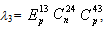

 . It is seen that population of the “empty” state 1 (without an electron) tends to unity (F1
 1) upon increasing the injection level. Population of the 3rd state decreases as F3 = λ3/(λ1n), and that of the NIRC-states 2 and 4 wanes in inverse proportion to n2: F2 = λ2/(λ1n2), F4 = λ4/(λ1n2). Limiting value of U is
 | (122) |
 , i.e. the rate of the GR-transitions becomes in inverse proportion to the number of injected carriers and carrier lifetimes increase proportionally to n2:τn≈τp≈n2/γ. As mentioned earlier, in this example fastest fading has been reached at bipolar carrier injection for the GR-transition rate through the defects with four states. In case of single polar carrier injection for defects with four states the rate U can wane even faster as PE-2. Let us show it on an example of the defect with 4-charge and without excited states. Suppose that only holes are injected into the sample, whereas concentration of free electrons remains constant or, maybe, decrease. The corresponding digraph G is shown in Fig.11e. The defect is “empty” in the 1st state and has one captured electron in the 2nd state. There are two and three captured electrons in the 3rd and 4th states, respectively. It is supposed also that the transitions 1
 2 and 2
 3 occur by electronic exchange only with the valence band. Only the transitions 3
 4 are due to exchange with both of the allowed bands. Since only hole concentration p plays the role of the PE, the digraph G has no NIRC’s and the ensemble will certainly be inertial. Only by one tree grows into each vertex determining the asymptotical behaviour of its tree-weight:
 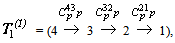 | (123) |
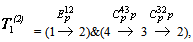 | (124) |
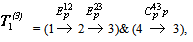 | (125) |
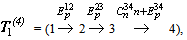 | (126) |
 | (127) |
 | (128) |
 | (129) |
 | (130) |
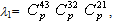
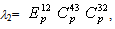
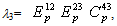
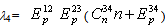 . With increasing the hole concentration more and more defects will occupy the “empty” RP-state,
  | (131) |
 | (132) |
 | (133) |
 | (134) |
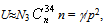 | (135) |
 n)/λ1, i.e. U drops in inverse proportion to p2. Thus lifetime of electrons and holes increase as p2: τn≈ (n/γ)•p2 and p3:τp≈p3/γ, respectively.Finally, 4-vertex digraph of states G is shown in Fig.11f, which corresponds to the defects with recombination rate U, equalling to zero at any injection conditions. Indeed, the digraph G contains three cycles:
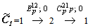
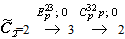 and
and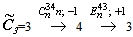 . In the above notations the arrows are the transition probabilities
  and the change of number of electrons in the conduction band
  is caused by this transition. Net change of number of free electrons along each cycle turns out to be equal to zero:
  , that is why U=0 (see, e.g., Eq.(50)).
5. Analysis and Discussion
- It should be noted that importance of the graph theory is much wider than being considered as one of the methods of studying the GR processes in semiconductors through point defects. The theory can be applied to any point defects with many numbers of states and with complicated transitions between them. The defects should be independent each from other and their kinetics should be possible to study by kinetic equations. Discrete approximation with any control-lable accuracy can be applied for many systems with continuous spectra of states. Examples of such systems are, e.g., extended defects, which can be described by the kinetic equations of Pauli, or Kolmogorov-Fokker-Planck equations, or integro-differential equation by Kolmogorov and Feller, accounting both continuous and abrupt change of the state of the system. This means that the distribution function and the rate of the GR processes for some extended defects with continuous spectra of states can also be built in the form of tree-weight rule similar to the discrete systems described by Eqs. (29)-(32). In such case, weights of the states should be calculated not by summation, but by integration over all oriented rooted spanning trees, entirely covering the strongly connected sink components of the continuous phase space. Here the integration over the oriented tree should be taken symbolically as a kind of limit that is associated with division of the phase space into small size cells, and in this respect, the integration along oriented tree is similar to the representation of the Feynman path integrals. These analyses indicate that the tree form of the state weights is the natural and inherent feature of any conservative linear system in steady state conditions, regardless of the features of the scheme allowed transitions, or features and the number of possible states of the system. By other words, it is the natural property of such systems. Knowledge of it allows to build the schemes of analysis of systems, which uses tree property of the weights of states.
6. Conclusions
- In the paper we have studied GR processes through point defects by the graph theory. In the theory the defect states will be indicated by dots whereas transitions between them as arcs. We show that in the description of the GR processes through point defects by the graph theory the principle of detailed balance can be accounted for by simultaneous including into consideration of both direct and reverse transitions between the defect states i and j (j→i and j←i ). We have classified defect models within the definitions of the graph theory and discussed why the theory present interest in the study of the GR processes. We found the equation for the stationary distribution function of the recombination centers on their states, which is universal for all point defects. We show that the equation can be derived without constructing the system of kinetic equations for the defect states and without solving the system of equations as it was done before by using the kinetic theory. We demonstrate that to find the distribution function of defects on their states it is sufficient to construct the set of rooted trees covering the digraph of states of defects G. We found that the graph theory can be supplementary to the kinetic theory by contributing to simplification of the model of the defects. If in the kinetic theory such a simplification is based on neglecting the defect transitions with smallest probability, by using the graph theory we demonstrate that it should be based not only on this, but also on strategically importance of the transition in the digraph of states of the defect. Also, we show that the graph theory can be efficient to find the equation for the distribution function of the defect on its states at asymptotic level corresponding to high injection level or temperature. It is based on dependence of the distribution function of defects on relatively small number of oriented trees of maximal weight, which can easily be determined by the methods of the graph theory. For that aim some transitions of the defect not included into any of the maximal trees determining asymptotical behaviour of the distribution function should be excluded from consideration. The distribution function itself can be very sensitive to some transitions of small probabilities included into maximal trees, but can be insensitive to other transitions with much greater probabilities and not included into the maximal trees. In graph theory this point is related to the concept of structural stability of dynamic systems. We show that the graph theory allows to construct the equation for the rate of GR processes. We have derived such an equation just using the digraph of states Gand without solving the system of kinetic equations. Distinct from already existing equations for the rate of GR processes, which work for particular type of the model of recombination, it is universal and works for all kinds of point defects. We show that such an equation can be derived without designing the system of kinetic equations and for that preliminary knowledge or derivation of distribution of defects on states for finding the equation for U is not needed. The rate U contains some terms, which are universal for all point defects and it allows the approximation
 , where
 and
and  are the excess electron(hole) concentration and lifetime. Based on the equation the rate of GR rate has been derived for some models of recombination via single level defects, excitonic states, bistable defects, and donor acceptor pairs. We show that the graph theory is efficient in formulation and solution of a wide range of challenges related to GR processes. We found the possibility of static influence of defects on GR processes without changing the charge state of the defect. It can take place together with the conventional astatic ones. We have revisited the problem of inertiality of recombination centers. In previous studies inertiality of recombination centers has been ascribed to number of energy levels of the centers, which is assumed to be more than one. Then delay in the GR processes could take place because of carrier exchange between the energy levels of defects. Here we have introduced different model of inertiality of the processes. We show that asymptotical dependence of U on carrier density at high injection levels can be found, whereas in the traditional approach it would be hardly possible to find so convenient criteria of lack of inertia. This work is the first attempt of systematic exposition of application of the graph theory in the study of GR processes considered mainly for point defects and it shows that the theory together with the kinetic approach is a new tool for investigation of GR processes.
ACKNOWLEDGMENTS
- The work was supported by Uzbekistan Academy of Sciences and Research Council of Norway.
Appendix A
- Let us deduce the Eqs.(12)-(15), which are on the base of the tree-weight rule from the matrix-tree theorem[1]. If the normalization condition for the distribution function has not been taken into consideration, then the components Fi (i= 1,…,M), in accordance with Eqs.(3)-(4), obey to the system of linear homogeneous equations
 | (A1) |
 . Off-diagonal elements wij of the matrix is equal to the probabilities ωji of transitions j
 i.
i.  | (A2) |
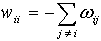 .Thus, all off-diagonal elements of the W-matrix are nonnegative, and the sum of all elements in any column is zero:
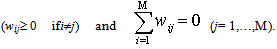 | (A3) |
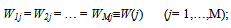 | (A4) |
 | (A5) |
 , which has only unities in the l-th row and coincides with the W-matrix in rest ones. All components of the column-vector
  except the l-th one, which is equal to unity, are equal to zero. Then using the Kronecker delta it is possible to write down
  ). Let us calculate the determinant of the B-matrix by decomposing it by the l-th row: detB =
  =
=  =
=  , and using equality of the cofactors Blj and Wlj of elements of the l-th row blj and wlj. Since among the magnitudes of W(j) there are non-zero ones and all of them, in accordance with the property 3), are of one sign, then detB ≠ 0 and the set of equations (A5) can be solvable:
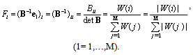 | (A6) |
 plays the role of the “kinetic weight” of the i-th state.Further, suppose that the system is described by the M-vertex digraph of states G. Kirchhoff’s matrix K(G) of the digraph G is the (MM)-matrix with i-th diagonal element kii equal to the sum of the weights of all the arcs coming into the vertex i. The off-diagonal element kij (i≠j) is equal to the sum (with minus sign) of the weights of all arcs issuing from the vertex j into the vertex i (see Ref.[1]). From this definition, in particular, it follows that all elements of the same row of the Kirchhoff’s matrix have identical cofactor. Let Ki(G) be a cofactor of the elements of the i-th row. According to the matrix-tree theorem, Ki(G) is equal to the total weight of all spanning trees, growing out of the vertex i. Proof of the theorem has been reported in Ref.[1, 2]:
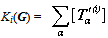 | (A7) |
 of the tree growing out of the vertex i serves to distinguish it from the tree
  growing into the vertex i. Weight of the growing out tree
 , as well as the one of the growing into tree, is equal to the product of weights of all arcs included into it:
 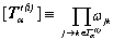 . Let us note now that the W-matrix and the Kirchhoff’s matrix K(G) are related with each other as:
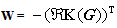 | (A8) |
 =[i]. Here we have taken into account that as a result of the operation ℜ, which changes orientation of all arcs into opposite ones, every tree
  growing out of a vertex i turns into the tree
  growing into the vertexi. Thus, the kinetic weight
  of the i-th state in Eq. (A6) coincides with the tree-weight[i] of the i-th vertex of a digraph of states G defined in Eqs. (12) and (13), and one gets the tree-weight rule Eqs. (12)-(15).It should be noted that upon deriving the Eq. (A6) it is supposed that at least one of the cofactors
  is not equal to zero. By virtue of the equality
  =[i] it means that the digraph G should have at least one “growing into” type of tree covering the digraph. Then the tree-weight of its root vertex will be different from zero. Also, it is equivalent to that in the digraph G. There should be at least one vertex accessible for all remaining ones. Only such a vertex can be a root for a tree[1]. For this purpose it is necessary and sufficient that the digraph G has only one strong component of sink type. Indeed, from the graph theory it is known that any digraph G has at least one strong component and each vertex of G belongs to the components. There are three types of strong components: (i) sink components denoted by A. It is possible to come into A and to leave it; (ii) source components (R). It is possible to leave R but it is impossible to come into it; transit components (T). It is possible to do both to come into T and to go out of it. Note that visual representation of possible transitions between strong components of a digraph G is provided by its condensation G*[3]. Any digraph G has one A-component, and if this component is unique, then each of its vertex will be accessible from any other vertex of the digraph G. Thus, starting from any vertex of the R-component, it is possible to pass through the vertices in T-components and to come back to the A-component, reaching there any vertex that is well visible on the example of the digraph shown in Fig. 11a. In this case each vertex of the A-component will be a root of at least one tree covering G. If number of the A-components is ≥2, then the vertices belonging to different A-components will be unreachable for each other, since there are no arcs outgoing from the A-components. Therefore, there will be no such vertices in G, which would be accessible from all others (see, for example, Fig. 11a) and no trees covering G. As discussed above, in this case the tree-weight rule is still valid but it should be applied not to the particular digraph G as a whole, but to each of its A-components separately, so that the rule takes on the form of Eqs. (29)-(32).It is also useful to analyse the above result from the other point of view of improving of understanding the question as to how the tree-construction of a vertex weight works. We want to show that only the weights defined by this way will provide the balance between the rates of the defects coming into any of their states and going out from the states at arbitrary variations of probabilities of transitions. Such a balance is necessary for achieving the steady state of the system. Solution of the set of Eqs.(3)-(4) expressing the balance must have the form of the tree-weight rule described by the Eqs. (12)-(15).First of all, we shall give some information about functional digraphs (see also Refs.1, 2). A functional digraph (to be called hereafter as Φ-digraph) represents a cycle C. Some trees, forming the so-called “forest”, may grow into the vertices of the cycle. Characteristic feature of aΦ-digraph is that exactly one arc outgoes from each of its vertex. If a tree growing into the vertex i will be added with an arc connecting the root vertex i with itself or with any other vertex j one gets aΦ-digraph and vice versa. The new arc will close a cycle C so that the root vertex i will appear in this cycle. The arcs, which have not been included into a cycle, generate the forest growing into the cycle. If an arc of a cycle C of aΦ-digraph has been excluded then one can get a tree growing into the vertex, which the removed arc was coming from. If aΦ-digraph contains all vertices and arcs of a digraph G, then one can say that the Φ-digraph covers G. Any strong digraph G can be covered with at least one Φ-digraph. Let us describe now two ways of constructing of all Φ-digraphs covering G and containing some fixed vertex i in their cycles C.First way. If a set of all trees {
  } covering G and growing into the vertex i is created, then each of them in turn without repetitions is combined with one of the arcs
  coming from the i-th vertex. As a result of each such association, one of the required Φ-digraphs will be gained, and in the end one can bust all the Φ-digraphs by one time each. It follows from the procedure that the total weight of the Φ-digraphs will be equal to
  , or
, or  . Weight of aΦ-digraph is equal to the product of the weights of all arcs included into it. This is the reason why the weight of the digraph can be presented as product of the weights of the trees included into it[
 ] by the weight ωij of an arc which is issued from the ith vertex.Second way. For all vertices j, distinct from i, and bound with it with an arc
  , the sets of all trees {
  } is created growing into them and covering G. Then each tree is supplemented with the ar
  which outgoes from its root j and comes into the vertex i. In the end one can again get the same set of Φ-digraphs. Such a way of construction allows one to write down total weight of the digraphs as
  , or
, or 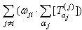 .Since in both of the above ways one gets the same result, it is possible to write down the following topological identity, which follows from properties of the spanning rooted trees:
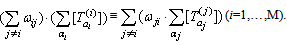 | (A9) |
 defined in Eqs. (12) and (4) provides automatically the equality of rates of transitions of defects from and into the state i:
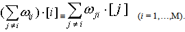 | (A10) |
Appendix B
- Let us prove the equality Un = Up at steady state conditions. For this purpose we shall make a difference of the rates Un and Up, which is equal to
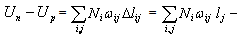
 [Eqs. (39),(40)]. Further, we interchange the indexes i
 j in the first sum:
 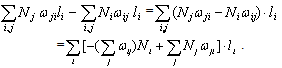 | (B1) |
 . Thus,
 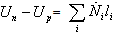 . It expresses the evident result that the difference between the capture rate of conduction electrons(holes) into the defects Un(Up) is equal to the rate of change of total number of electrons bound on the defects. In the steady state conditions
  = 0 for all i = 1,…,M. Hence Un = Up.
Appendix C
- We shall deduce the equation for the rate of GR-transitions[Eq. (46)] by using the Eq. (38). For this purpose we shall write the density of defects Ni in the i-th state via the tree-weights of the vertices of the digraph of states G: Ni = Ntot•[i]/
 . Here the tree-weight[i] is obtained by summing the weights of all the trees covering G and growing into the i-th vertex:[i] =
  . Thus, the Eqs. (39) and (40) become
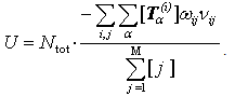 | (C1) |
 growing into the i-th vertex with an arc i
 j issued from its root vertex i gives some Φ-graph
  covering G and that the product[
 ]•ωij gives the weight[
 ] of this Φ-graph. Note that adding the arc
  closes the cycle Ck together with remaining arcs of the tree
 , not included into this cycle, constitute the Φ-graph
  . Thus, each addend in the numerator of the fraction (C1) represents product (taken with minus sign) of the weight of some Φ-graph
  by the change of the number of free electrons corresponding to some arc belonging to its cycle Ck. Since the summation in the numerator of eq.(C1) is carried out over all trees, and since for each of them all possible variants of association with the arc are considered, then it will contain the weights of all Φ-graphs covering G. It is easy to understand that the weight of each Φ-graph
  will meet as many times as many arcs are there in its cycleCk, and every time it will be multiplied by the number νij corresponding to the next arc of the cycle. Combining the addends with one and the same weight[
 ] together, one can get the factor νk, which is equal to the net change of the number of free electrons along the cycle Ck of the Φ-graph
  and we obtain the Eq. (46).
Appendix D
- Let us show that in the absence of degeneracy, the rate of GR-transitions can be calculated by the Eq. (51) provided that the model together with each transition holds its reverse transition. Let the probability
 of transition of a defect from the i-th state into the j-th state by some particular mechanism αis
 . As is known, in absence of degeneration the exponents
  and
and  coincide with number of free electrons and holes involved in the transition, respectively. As a result of the transition, number of free electrons varies by
 . In accordance with Eq. (51), number of holes will be varied by
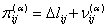 . Note that the number of free electrons
  participating in the transition and the change of
  in the conduction band
  due to the transition not necessarily should coincide with each other. Another example is the Auger-process shown in Fig.7c, in which one free electron participates:
  = 1, but the number of conduction electrons does not vary:
  = 0. The same concerns to the quantities
  and
and . Transition probability of a defect from the jth state into the ith state by the reverse mechanism
  will be
 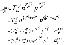 | (D1) |
 and
and  respectively, and it will be the initial parameter for the reverse transition by the
  -mechanism. The ratio of the coefficients
  can be found from the principle of detailed balance: since in equilibrium the rates of transitions by mutually reverse mechanisms equilibrate each other, i.e.
 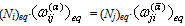 | (D2) |
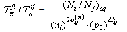 | (D3) |
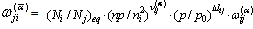 | .(D4) |
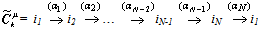 passing through N different vertices i1, i2,…,iN1, iN, with arcs α1, α2,…,αN corresponding to different mechanisms. As discussed above, the cycle belongs to the kth subgroup of cycles passing through the vertices in certain order and differing each from other by choice of the multiple arcs, i.e. by the mechanisms of transitions, and in this subgroup it will be characterized the number μ. Its weight will be equal to
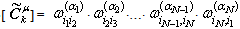 . Since each transition comes with the reverse one, the digraph G contains another cycle
 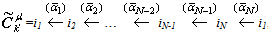 , which will pass through the same vertices as
 , but in the opposite direction corresponding to reverse mechanisms of transition. The cycle will belong to the group
  and will have the number
  . By using the Eq. (D1) one can find the relation between the weights of the two mutually reverse cycles
  . Here
  is the total change of number of the free electrons along with the cycle
  because upon cyclic multiplication both (Ni/Nj)eq and
  equals to 1, and degree in the power of the equation
  , being added will equal to
  . At the same time it is evident that change of number of electrons in the conduction band occurring in the mutually reverse cycles are opposite as well
 , because they contain the mutually reverse mechanisms. Therefore the net contribution from the two mutually reverse cycles to the numerator of the Eq.(50) will be equal to
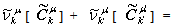
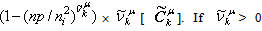 ,then it can be represented as
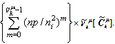 Then the Eq. (50) becomes of the form of Eq.(51).
Appendix E
- Upon proving equality of the rate of GR-transitions Ueq to zero at equilibrium one should bear in mind that the digraph of states G describing the system must be symmetrical. Thenthe principle of detailed balance will be fulfilled, which requires that a reverse transition for each of the direct transition. Since a symmetrical digraph Gwith a cycle Ck always contains a counter cycle
 , which passes through the same vertices as Ck, but in the opposite directions, all cycles of such a digraph can be divided into pairs of mutually reverse cycles. For this reason all Φ-graphs covering G can be divided into pairs
  and
and , which will differ each from other only by orientation of their cycles. However, these cycles will have the same sets of trees growing into them. In equilibrium state weights of the mutually reverse cycles are equal, which follows from the principle of detailed balance:
 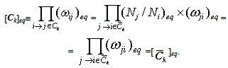 | (E1) |
 whereas changes of the numbers of free carriers along the cycles Ck and
  will be opposite
  . Indeed, the mutually conjugate cycles Ck and
  include the mutually reverse mechanisms of transitions α and
  which cause the opposite changes in number of free carriers in allowed bands:
  . Therefore,
 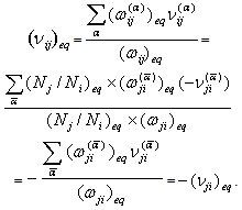 | (E2) |
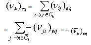 | (E3) |
 and
and  from the Φ-graphs containing the counter cycles are mutually cancelled and the Eq. (46) is reduced to the equality Ueq= 0.
Appendix F
- Let us show that the least possible magnitude of the exponent d in asymptotic dependence U ∝PEd in absence of degeneration and Auger processes is equal to s – M + 1. Here M is the number of the different states of a defect. s = 2 for bipolar and s = 1 for single polar injection. Indeed, the tree of maximal weight T covering the M-vertex digraph G will have an asymptotical weight[T] ∝PEt, for which the exponent t may reach the maximal possible value M – 1, i.e be equal to the number of the arcs of the M-vertex tree, if the weight of each arc will be proportional to PE1. This is the largest possible degree for the denominator in Eq.(50). At the same time, the smallest possible degree for the numerator coincides with the value of the above-mentioned parameter s. Really, the cycle
 with non-zero
 , should, of course, contain at least two transitions. One of them should be the electron capture from the conduction band and the another one should be the hole capture from the valence band. Therefore weight of the cycle containing the product of probabilities of the two transitions will contain a factor PEs. Weights of remaining arcs of the cycle will be proportional to PE0 and PE1. Therefore, exponent for the cycle weight cannot be smaller, i.e. min deg[
 ] = s. The smallest degree for the weight[
 ] is equal to zero. It takes place when weights of all arcs forming the set of forests
  are proportional to PE0: min deg[
 ] = 0. Then, according to Eq.(32), min deg U = min deg[
 ] + min deg[
 ] – max deg[T] = s + 0 – (M – 1). This is what has been stated above.