-
Paper Information
- Next Paper
- Paper Submission
-
Journal Information
- About This Journal
- Editorial Board
- Current Issue
- Archive
- Author Guidelines
- Contact Us
American Journal of Condensed Matter Physics
p-ISSN: 2163-1115 e-ISSN: 2163-1123
2013; 3(3): 31-40
doi:10.5923/j.ajcmp.20130303.01
Study on Electron/Positron Scattering in Solid Targets Using Accurate Transport Cross-sections: Comment on Z. Rouabah et al Papers
 Abstract
 Reference
 Full-Text PDF
 Full-text HTML
A. Bentabet1, A. Betka2, A. Azbouche3, N. Fenineche4, Y. Bouhadda5
1Laboratoire de Caractérisation et Valorisation des Ressources Naturelles (LCVRN), université de Bordj Bou-Arreridj, 34000, Algeria
2Départements de physique, faculté des sciences, université de Sétif, 19000, Algérie
3Nuclear Research Center of Algiers, 2 Boulevard Frantz Fanon Alger, Algeria
4IRTES-LERMPS/FC LAB, UTBM University, Belfort, France
5Unit of Applied Research in Renewable Energy, 47000, Ghardaïa, Algeria
Correspondence to: A. Bentabet, Laboratoire de Caractérisation et Valorisation des Ressources Naturelles (LCVRN), université de Bordj Bou-Arreridj, 34000, Algeria.
| Email: |  |
Copyright © 2012 Scientific & Academic Publishing. All Rights Reserved.
We should be very careful, when we applied a combination between two models, especially if the first one is stochastic (probabilistic) and analytic (deterministic) for the second , which is the case of the papers of Rouabah et al[Appl. Surf. Sci. 255 (2009) 6217 and Appl. Surf. Sci. 256 (2010) 3448]. In fact, this work has an aim to show the valuable approaches to study the transport of electron/positron in solid target. Our work is presented as a comment on the papers of Rouabah et al. Indeed, after mentioned some weak points of Rouabah et al works we have discussed different points: the screened Born transport cross-section (TCS) and the true model of Jablonski[Phys. Rev. B 58 (1998) 16470], the large deviation between Rouabah et al TCSs and the accurate values, the combination between Monte Carlo simulation and Vicanek and Urbassek theory[Phys. Rev. B 44 (1991) 234] and the normalization condition as well. Besides, we have given some recommendations on the range calculation using Monte Carlo method.
Keywords: Electron Scattering, Positron Scattering, Transport Cross-Sections, Electron Range, Monte Carlo Simulation, Deterministic Model, Range of Penetration
Cite this paper: A. Bentabet, A. Betka, A. Azbouche, N. Fenineche, Y. Bouhadda, Study on Electron/Positron Scattering in Solid Targets Using Accurate Transport Cross-sections: Comment on Z. Rouabah et al Papers, American Journal of Condensed Matter Physics, Vol. 3 No. 3, 2013, pp. 31-40. doi: 10.5923/j.ajcmp.20130303.01.
Article Outline
1. Introduction
- The electron and positron material interaction has a great importance in several domains of the analytical techniques of the material such as electron probe microanalysis, electron energy-loss spectroscopy, Auger electron spectroscopy, positron annihilation spectroscopy, etc. Electron-transport calculations are usually performed by means of either analytical theory or Monte Carlo simulation. It is important to know that the latter (Monte Carlo method) has become a powerful tool in the calculation and prediction of radiation effects in the solids. Both methods require an accurate knowledge of the cross-section for elastic scattering of electrons as functions of the projectile kinetic energy E. For that reason, Rouabah et al[1-3] have been interested to propose a simplified expression of the transport cross-section of electron and positron by basing on analytical expression reported by Jablonski[4]. The direct calculation of the deviation between their interpolated results and the accurate values shows that there are drastic deviations. In addition, Rouabah et al have combined between the Vicanek and Urbassek theory[5] (deterministic model) and the Monte Carlo simulation (probabilistic model) to investigate the transport of 0.5–4keV electrons in solid targets[1, 6]. However, when we applied a combination between two different methods we should be very careful especially if the first model is stochastic (probabilistic) and the second is analytic (deterministic). After a careful analysis of Refs.[1-3, 6-8] we notice that there is an abnormal problem in number of questions: the expression of the electron TCS[1-3], the combination between Monte Carlo and analytic model[1, 6], the backscattering coefficient results[1,6-8], the range of penetration[1, 6-8] and the large deviation of their results[1-3, 6-8]. Moreover, some errors are repeated in all Rouabah’s papers[1-3, 6-8] (see below). We note that we have focused our attention on Rouabah’s paper “[1]” which was the base of number of their other works. So, the present work shows necessary considerations to study the transport of the slow electrons and positrons in solid targets.This paper is organized as follows. In Section 2 we describe our comments on the methods used in the calculations: the transport cross-sections, the normalized combination between the Monte-Carlo simulation and the Vicanek and Urbassek theory, the electron range, the mean number of wide angle collisions and the analytical backscattering coefficient. Finally, Section 3 contains the conclusion.
2. Methods and Comments
- Our comment on the Rouabah et al works could be summarized on three subjects: their transport cross-section (TCS), their combination between analytic and stochastic models and their calculated range using Monte Carlo method.
2.1. Comment on Rouabah et al TCSs
- Rouabah et al suggested a simplified expression of the electron transport cross section using a simple fit. However, actually, they have attributed in their work[1-3, 6-8], an old screened TCS (denoted
 ) to Jablonski[4]. Indeed, firstly, we will present the demonstration that
  is more than 60 years old; then we present the true Jablonski TCS.
2.1.1. The Screened Cross Sections and The Wentzel Model (1927)
- According to Fernandez-Varea et al[9]: “The Wentzel[10] approach for describing elastic scattering of particles with charge Z'e (Z ' =- 1 and + 1 for electrons and positrons, respectively) by atoms of atomic number Z is based on the simplified scattering potential
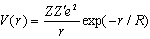 | (1) |
 | (2) |
 is the Bohr radius (
 ) and
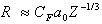
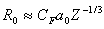
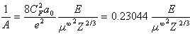
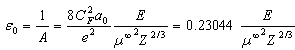
) and  . “However, it is more expedient to determine R so as to obtain agreement with more accurate elastic scattering cross sections”[9].Generally, R has been taken using the next form (see Nigam[11] (1959)):
 | (3) |
 and µ is a constant (generally µ>1 which signifies that
  ).It could be noted that, at high incident electron energies we take µ = µ∞[12]. Moreover, the first order Born approximation is valid only at that case (see below). Thus:
 | (4) |
 depends on the used screened potential and the energy[12]. For example, some authors take
  as value corresponding to the Thomas Fermi potential (i.e.
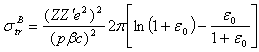
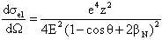
 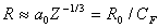 see[11-14]). The transport cross section corresponds to the screened Differential Cross Section (DCS) (which is obtained from the first order Born approximation), which gives[9]
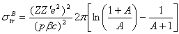 | (5) |
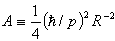 | (6) |
 ), the equation (6) can be rewritten as follows:
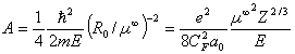 | (7) |
 | (8) |
 ,
,  | (9) |
 | (10) |
 can be rewritten as follows:
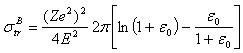 | (11) |
 | (12) |
 | (13) |
 attributed by Rouabah et al to Jablonski[4]. Consequently the age of
  is more than 60 years old (since the works of Wentzel (1927) and Nigam 1959). We note that Rouabah et al have repeated this error (the attribution of
  to Jablonski[4]) in all their works[1-3, 6-8 ]. Consequently, all these works must be reviewed.
 2.1.2. The Demonstration that the TCS Derived by Jablonski[4] is not 
- We recall that Jablonski said in his abstract[4]: “Analytical description of photoelectron and Auger-electron transport in solids requires values of the transport cross sections
 for electron energies between 50 and 2000 eV. An analytical formula is proposed to provide needed values of
  for energies in this range and for all elements.” To proof that
  derived by Jablonski[4] is not
  we can base on Jablonski “himself”[4] as follows:1. The great proof is the above calculations (see above “section I”). 2. The symbolization differences between
  and
and  : Jablonski[4] used the symbolization
  in the Abstract, equations: (2[definition], 21,24a, 25, 27, 32 ..) however he used the separate symbolization
  (i.e. without multiplying it by
  ) only in equations (8 and 15) and he don’t use it in his results section.3. The index B in
  : Jablonski (himself) said[4]:“the index B denotes the first-order Born approximation.”4. The index “∞” in
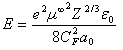
  which signifies “At sufficiently high incident electron energies[12]”, which is not the case of Jablonski study[4] {50-2000 eV}. Knowing that Jablonski himself said[4]: “ The constant µ in the screening parameter
  depends on energy, especially at energies below 1 keV. The use of the asymptotic value µ∞ is justified only at energies exceeding 5 keV”. 5. The calculated deviation mentioned in Jablonski abstract[4] correspond to
  (see equation (27) in Jablonski paper[4])6. We note that the index B of
  denotes first order Born approximation. However, the first order Born approximation is not valid at lower energies (see[4]; E must verify
  ; thus, the electron energy should exceed 229.2 eV for carbon or 1277.7 eV for gold) which is not the case, too, of 50-2000 eV especially for heavy atoms. In addition Jablonski himself said[4]:“Thus, the accuracy of the first-order Born approximation for
  is generally rather poor. To obtain a more accurate analytical expression for
  , we need an additional analytical function G(ε0) correcting the cross section
  ”.7. We recall also that Jablonski (himself) said[4]:”An improved analytical expression is derived here to provide reasonably accurate values of
  in the energy range of interest for surface-sensitive electron spectroscopies, i.e.,50–2000 eV.” We note that the deviation of
  by comparison to that obtained by quantum methods reached drastic values. In Table 1 we presented
  ,
,  (tabulated by Mayol and Salvat[15] who used the Relativitic Partial Waves Expansion Method (RPWEM)) and the percentage deviation between them. For example, we remark that at E=250 eV the percentage deviation of
  reaches ≈1500 % for Au (Z=79). Has Jablonski proposed such approximation and said “…reasonably accurate values of
  ..”? 8. In the abstract of[4], Jablonski said: “For atomic numbers up to 30, the mean deviation between accurate values of
  and values from the analytical formula reaches 0.5%. For several elements with larger atomic numbers, this deviation increases to 5%, although it is much lower for the majority of cases” . However, from Table 1, we can remark that the deviation of
  is always greater than 2%. Moreover, we found that the deviations reached drastic values: 30%, 50%, 200 %, 1500%,.. Consequently, and certainly,
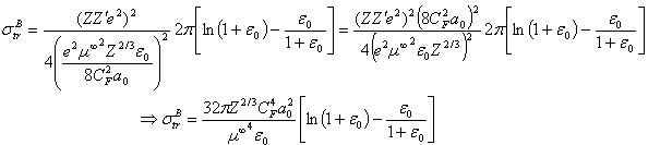
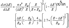
  is not the TCS mentioned in the abstract of Jablonski paper[4].Actually the TCS derived by Jablonski lies in his paper[4]: “Thus, the accuracy of the first-order Born approximation for
  is generally rather poor. To obtain a more accurate analytical expression for
 , we need an additional analytical function
  which correcting
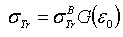 | (14) |
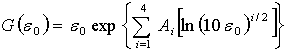 | (15) |
2.1.3. Rouabah et al TCS[1]
- Before quoting our point of view of this section, we recall that Rouabah et al used the same transport cross section expressed by equation (13) where the only difference is that
 has been taken as a free parameter. Thus, to determine
 , they have adjusted
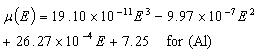
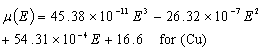
  to Mayol et al TCS[15]. After a fitting process, they suggested the next interpolation form of
  given by:
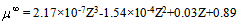 | (16) |
 to
to  [15]; by basing on the equation (13), it is easily to conclude that "μ∞" is given by:
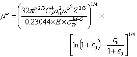 | (17) |
 depends implicitly on the energy (as example), we should find a relation between at least one parameter (x or y ..) depends explicitly on the energy otherwise
  is independent explicitly and implicitly on the energy. For example, if
  and
and  we can said that f(x,y,..) depends explicitly on x and implicitly on E. Indeed, the equation (16) does not any relation with the energy; neither explicit nor implicit. ● Rouabah et al[1] have adjusted
  to
to  [15]. So, the large deviation between them (see below) is the proof of the weak point of this choice. ● Elsewhere, we note that the TCS results of[1] (denoted by
  in their tables (1-4)[1]) don’t correspond to their fit given by equation (16). After a number of tests we think that they have used the next expression:
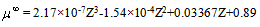
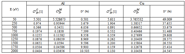
2.1.4. The invalidity of Rouabah et al TCS[1]
- To show that Rouabah et al TCS fit[1] is not accurate, we can based on their data results themselves. In fact, Table (2) represents their TCS[1], Mayol and Salvat TCS[15] and the percentage deviation between them. We think that, these deviations are clearly invalidates their proposal fit (for Al: 21% and 12 % at E=250 and 500 eV… respectively, for Cu: 41%, 20% and 10.2 % at E=250, 500 and 1000 eV respectively, for Au: 96% and 30.3 % at E=250 and 500 eV respectively ….). Unfortunately, this Rouabah et al TCS[1] has been used in other Rouabahah’s papers[1, 6-8]. Consequently all their works[1, 6-8] must be reviewed and revised.
2.1.5. The invalidity of Rouabah et al TCS[2]
- Rouabah et al[1], in order to show that their model[1] is valid, have presented three tables carrying out a comparative study: their TCS (
 )[1], TCS of their previous work (
 )[2],
)[2],  given by equation (13) and the TCS tabulated by Mayol and Salvat (
 )[15] where it is clear that
  is in better agreement with
  than both
  and
and . By contrast, this latter is not the proof of the validity of their fit[1], but it is the proof of the invalidity of
  [2] and
 . Concerning the invalidity of
  at lower energies; it has been discussed above. However, the invalidity of their
  “[2]” can be proved as follows:Rouabah et al carried out an erratum[16] on their results of[2] in which they precise[16]:“(i) in all the text, the statement percentage deviation has to be replaced by relative deviation. (ii) In table (4) and fig.1, the deviations D and D’ are expressed in absolute units and not as percentages.”. We think that it will be better that if the table (4) and Fig. 1 of[2], expressed as percentage commonly used in literature (i.e. more appropriate than absolute units). So, to prove that the TCS of[2] is inaccurate, we can combine between their results published in[2] and their erratum[16]. Take for example their table (4) of their work[2], the colon D (which corresponds to the deviation of their results) of Au (Z=79) we find the next results: 4.62, 1.61, 0.49, 0.29, 0.16, .. According to their erratum[16] “the deviations D are expressed in absolute units and not as percentages” so, these values (4.62, 1.61,…) are in absolute units; by consequence these deviations become in percentage as follows: 462%, 161%, 49%, 29%, 16% .. These deviations are totally unacceptable for the fitting process. Indeed, we should multiply their published deviations by 100 (on other word the error factor is 104%). Consequently, we note and we reconfirm that their erratum[16] also invalidates their work[2].
2.1.6. The Invalidity of Rouabah et al TCS[3]
- Rouabah et al[3] repeated approximately the same above mistake of[1] in the case of positron. After an adjustment process to Dapor results[17], they are suggested two interpolation forms of
 given by:
 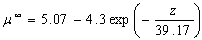 | (18) |
 | (19) |
2.2. The Combination between Monte Carlo Simulation and Vicanek And Urbassek Formula
- Before giving our point of view; we recall that Rouabah et al[1] have used Monte Carlo simulation (MC) to calculate the range and Vicanek and Urbassek formula to calculate the backscattering coefficient (BSC). In their MC simulation they used the screened Rutherford cross section, given by:[18]
 | (20) |
 | (21) |
 | (22) |
 in the following) obtained by integrating
  is given by:
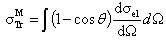 | (23) |
 ) is expressed as[5],
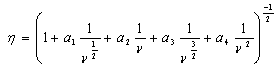 | (24) |
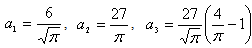 and
and .In relation (24),
  is the mean number of wide angle collisions defined as,
 | (25) |
 is the transport cross-section,
  is the range of penetration and
  is the number of atoms per unit of volume in the solid target given by:
 | (26) |
 and A are the Avogadro number, the density and the atomic mass of the target respectively.So, to calculate
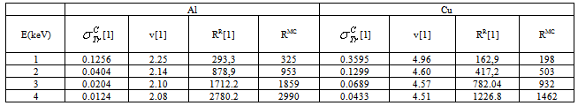
  , Rouabah et al[1] used MC simulation to calculate the range and for this raison, they think that they have carried out a combination between MC simulation and Vicanek and Urbassek formula. We think that the word “combination” is not appropriate because, we think that to do a combination between MC and the analytic model; the authors of“[1]” should be used the same elastic and inelastic models (i.e. the same input data). To show that the authors of[1] have not carried out a normalized combination, we have presented in Table (4)
  and
and  where we remarked a big difference between them (i.e. the TCS used by[1] in Vicanek and Urbassek expression do not correspond to that obtained by integrating
  used by them in their MC code).Besides, is this combination between Monte Carlo method and Vicanek and Urbassek theory evident and realistic? Most part of the response is mentioned in our paper[19]. Indeed, we have showed that: firstly, the Monte Carlo method is more recommended, generally, to be used in the calculation of the backscattering coefficient than Vicanek and Urbassek theory (with a condition to use the same input data)[19].Consequently, we did not need to use this combination. Secondly, the use of this combination should be done by taking into account the normalization condition[19]. To make clear the normalization problem, we can give the following example:Let’s note by N0, Na and Nb: the incident particles number, the absorbed particles number and the backscattered particles number. We suppose that N0=10 (to facilitate calculations)We suppose also that Monte Carlo method gives backscattering coefficient BSC1=0.3 (so we conclude that in this case Nb=3 and Na=7), and their model (combination between Monte Carlo and Vicanek and Urbassek model) gives BSC2=0.2 (so we conclude that in this case Nb=2 and Na=8). Now, if we take BSC2 as a reference for calculations (accurate results), the absorbed particles number is 8, but when we use Monte Carlo, Na is 7. Consequently, this is a contradiction: which is the correct 7 or 8? The problem of the normalization becomes very difficult when the target is a thin film[19] which is the case of their paper[6].Consequently, both their works[1, 6] must be reviewed. Moreover, we note that Rouabah et al[6] have used the Vicanek and Urbassek formula to calculate the backscattering coefficient in function of the film thickness. Let’s ask a question: who showed that the mathematical expression of the backscattering coefficient developed by Vicanek and Urbassek (equation (24)) is applicable for thin films? Knowing that this formula is valid only for semi-infinite solid case or for thin film with a thickness for which we can consider it as a semi-infinite solid. We note that Vicanek and Urbassek said -as example- the next clear expression “The present scheme has to be completed by semi-infinite medium boundary condition[5]”. This latter is the second proof of the no evidence of their BSC results in function of the film thickness, in one hand, and the equation (24) is not applicable for thin films, in another hand.
 2.3. The Electron Range, the Mean Number of Wide Angle Collisions and the Backscattering Coefficient Results
- Rouabah et al[1] used Monte Carlo simulating individual electron scattering events where the elastic model is that given by equations (20-22) and the inelastic processes are handled in terms of Gryzinski`s excitation function[20]. The Gryzinski`s differential cross section is given by,
 | (27) |
 ,
,  , and E are the energy loss, the mean electron binding energy, and the primary projectile energy, respectively.The electron range (R) calculated by Rouabah et al[1] can be deduced by using their data tables[1]. So, from the equations (25-26) we conclude that R can be written as follows:
 | (28) |
 | (29) |
 | (30) |
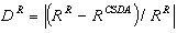
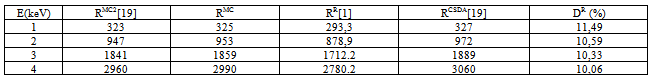
 where E0 and S(E) are the primary energy and the stopping power of primary particle respectively. The integration was performed, generally, from the primary energy E0 to the cutoff energy instead of 0 eV.Indeed, we note that in our work[19] we have calculated the range using CSDA for Al. So, Table (6) represents their range (RR), the range by using the same code (RMC), the range using CSDA (RCSDA) and the deviation between them. We note that Rouabah et al[1] have taken 20 eV as a cutoff energy however the RCSDA calculated by[19] has been done for the cutoff energy equal to 100 eV. Consequently, when we added the range between 20 eV to 100 eV the deviation becomes greater (reaches ≈13 % for E=2keV). Therefore, on the basis of Jablonski et al notification, while the deviation is more than 10% (particularly for E>1 keV) then the results of[1] are incorrect. Consequently, all their results concerning the mean number of wide angle collisions and the backscattering coefficients are incorrect. We note that this error has been repeated by Rouabah et al in their work[6]. By consequence, both their works[1, 6] must be reviewed.Important remarks:■ We are recognized that the notification “to say that the algorithm range is true it must be no deviations between the ranges obtained analytically and that obtained by using CSDA in Monte Carlo scheme otherwise the used Monte Carlo code is wrong (except a statistical fluctuation, due to the use of the Monte Carlo simulation)” was the notice of the reviewer chosen by the Journal Nucl. Instrum. Methods Phys. Res. B to review the paper[19]. We think that this notification is the key to confirm the validity of the Monte Carlo Algorithm range.■ In the case of the Monte Carlo method the statistical fluctuation error is calculated as
  , where N is the number of initial particles[22]. Since 104 particle histories were used by the authors of[1], this statistical error is found to be about 1%. On other words, the deviation of their ranges[1, 6] is not due to the statistical fluctuation but there is an error calculation.
3. Conclusions
- In summary, in this comment we have showed that Rouabah et al transport cross sections are inaccurate and in reality were not based on Jablonski’s[4], as well. Moreover, their combination between Monte Carlo and Vicanek and Urbassek theory is not normalized and all their results concerning the mean number of wide angle collisions and the backscattering coefficients must be reviewed and revised. In other words, our work about Rouabah et al papers[1-3, 6-8, 16] can be summarized by point as follows:1.
 (Transport cross section) attributed in[1-3, 6-8] to Jablonski[4] is not true, but it is an old cross-section.2. Actually the transport cross section of Jablonski[4] is that given by
  3. The tabulated results of
  (their tables 1-3 of[1]) do not correspond to their fit by using:
 4.
4.  Depends on Z and E but not only on Z. 5. The passage from
  depends on Z and E to
  depends only on Z is not justifiable, if is not impossible.6. The deviation of (15 %.., 20%,.., 25%, ..30%,...40%, …) shows clearly the invalidity of their fit[1-3]. 7. The combination between Monte Carlo and Vicanek and Urbassek theory has been used without a normalized manner[1, 6]. 8. The ranges calculated by Rouabah et al[1, 6] are not correct.9. The mean number of wide angle collisions of Rouabah et al are not correct[1].10. Some (if it is not all) their backscattering coefficients [1, 6-8] are not correct.11. We recall that Rouabah et al have calculated the range by using Monte Carlo simulation where they used the screened Rutherford cross section and the Gryzinski model to describe the elastic and inelastic collisions respectively. We confirm that either by using CSDA or scattering by event of Monte Carlo schemes, the range calculated by Rouabah et al[1, 6, 8] do not correspond to the true values (of Gryzinski range).12. Their erratum[16] itself invalidates their work[2].
 to
to  . D: is the deviation.
 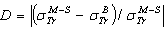 .
. : The electron transport cross section tabulated by Mayol and Salvat[15].
  : TCS of Born approximation given by (13) with µ∞=1.22
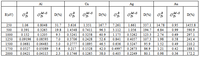
|
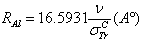
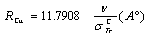
 to
to  in function of Z expressed in A˚ 2.
  : The electron transport cross section tabulated by Mayol and Salvat[15].
  : The electron transport cross section tabulated by[1].
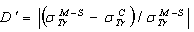
|
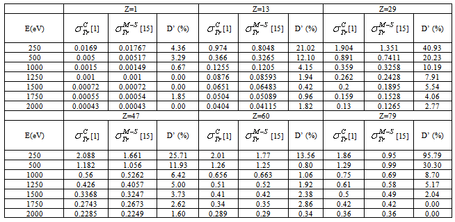
 : Rouabah et al TCS given by (13, 18)[3].
  : Rouabah et al TCS given by (13, 19)[3].
  Dapor TSC[17]. D1: percentage deviation between
  and
and  . D2: percentage deviation between
  and
and 
|
 : Present work by using the elastic model of[18].
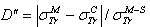
|
|
References
| [1] | Rouabah, Z., Bouarissa, N., Champion, C., Bouaouadja, N., 2009, Study on electron scattering in solid targets using accurate transport cross-sections, Appl. Surf. Sci., 255, 6217-6220. |
| [2] | Rouabah, Z., Bouarissa, N., Champion, C., 2009, Improved expression for calculating electron transport cross sections, Phys.Lett.A, 373, 282-284. |
| [3] | Rouabah, Z., Bouarissa, N., Champion, C., Bouzid, A., 2010, Calculation of transport cross sections for positrons in solid targets via improved expressions, Sol.Stat.Comm., 150, 1702-1705. |
| [4] | Jablonski, A., 1998, Transport cross section for electrons at energies of surface-sensitive spectroscopies, Phys. Rev. B, 58 (24), 16470-16480. |
| [5] | Vicanek, M., Urbassek, H.M., 1991, Reflection coefficient of low-energy light ions, Phys. Rev. B, 44 (14), 7234-7242. |
| [6] | Rouabah, Z., Bouarissa, N., Champion, C., 2010, Electron impinging on metallic thin film targets, Appl. Surf. Sci., 256, 3448–3452. |
| [7] | Rouabah, Z., Bouzid, A., Champion, C., Bouarissa, N., 2011, Electron range-energy relationships for calculating backscattering coefficients in elemental and compound semiconductorsSol.Stat.Comm., 151, 838-841. |
| [8] | Bouzid, A., Rouabah, Z., Bouarissa, N., Champion, C., 2012, Penetration range and backscattering ratio of low-energy electrons in metals, J. Electron. Spectrosc. Relat. Phenom., 185, 466– 469. |
| [9] | Fernhndez-Vareaa, J.M., Mayola, R., Barob, J., Salvat, F., 1993, On the theory and simulation of multiple elastic scattering of electrons, Nucl.Instr.Method.B, 73, 447-473. |
| [10] | Wentzel, G., 1927, Z. Phys., 40, 590. |
| [11] | Nigam, B. P., Sundaresan, M. K., Wu, T.-Y., 1959, Theory of Multiple Scattering: Second Born Approximation and Corrections to Molière's Work, Phys. Rev. 115, 491-502. |
| [12] | Jablonski, A., 1981, Approximation of atomic potentials by a screened Coulomb field, J. Phys. B: At. Mol. Phys., 14, 281-288. |
| [13] | Liljequist, D., Salvat, F., Mayol, R., Martinez, J. D., 1989, Simple method for the simulation of multiple elastic scattering of electrons, J. Appl. Phys., 65 (6), 2431-2438. |
| [14] | H. E. Bishop, 1967, Electron scattering in thick targets, J. Appl. Phys., 18, 703-715. |
| [15] | Mayol, R., Salvat, F., 1997, At.Data Nucl. Data Tables, Total and transport cross sections for elastic scattering of electrons by atoms, 65, 55-154. |
| [16] | Rouabah, Z., Bouarissa, N., Champion, C., 2009, Erratum to: “Improved expression for calculating electron transport cross sections”[Phys. Lett. A 373 (2009) 282], Phys.Lett.A 373, 1599. |
| [17] | Dapor, M., 1995, Nucl. Instrum. Methods Phys. Res. B 95, 470-476. |
| [18] | Bouarissa, N., Deghfel, B., Bentabet, A., 2002, Electron slowing down in solid targets: Monte-Carlo calculations, Eur. Phys. J: Appl. Phys., 19, 89–94. |
| [19] | Bentabet, A., 2011, the range of penetration and the backscattering coefficient by using both the analytic and the stochastic theoretical ways of electron slowing down in solid targets: Comparative study, Nucl. Instrum. Methods Phys. Res. B, 269, 774 –777. |
| [20] | Gryzinski, M., 1965, Classical Theory of Atomic Collisions. I. Theory of Inelastic Collisions, Phys. Rev. A, 138, 336-358. |
| [21] | Jablonski, A., Powell, C.J., Tanuma, S., 2005, Monte Carlo strategies for simulation of electron backscattering from surfaces, Surf. Interface Anal., 37, 861 – 874 |
| [22] | Zommer, L., Jablonski, A., Gergel, G., Gurban, y S., 2008, Monte Carlo backscattering yield (BY) calculations applying continuous slowing down approximation (CSDA) and experimental data, Vacuum, 82, 201 –204. |
| [23] | Bentabet, A., Fenineche, N., 2009, backscattering coefficients for low energy positrons and electrons impinging on bulk solid targets, J. Phys.: Condens. Matter, 21, 095403 (5pp). |