1. Introduction

The RFIM has been extensively studied due to its interest as asimple frustrated system, as well as its close connection toexperiments[1]. Its beauty is that the mixture ofrandom fields and the standard Ising model creates rich physicsand leaves many still unanswered problems. The Hamiltonian describing the model is

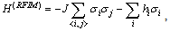(1)

whereare Ising spins, is thenearest-neighbour's ferromagnetic interaction, and areindependent quenched random fields obtained from a relevantdistribution. Although the existence of anordered ferromagnetic phase for the RFIM is wellestablished, many years now[2], a clear resolution ofits critical behaviour is still lacking, in many terms.Historically, one of the main puzzles has been the mean-fieldprediction of a tricritical point in the phase diagram of thebimodal RFIM[3]. Currently, although we know thatthe phase transition of the RFIM is of second – orderwith a verysmall value of the exponent β, irrespective of [3-7], alarge controversy on the scaling behaviour of the specific heatcontinues to castdoubts[4,8-13].

In particular, the specific heat of the RFIM can be experimentallymeasured[8] and is, for sure, of great theoreticalimportance. Yet, it is well known that it is one of the mostintricate thermodynamic quantities to deal with in numerical simulations,even when it comes to pure systems. For the RFIM, Monte Carlomethods at positive temperatures have been used to estimate the value of itscritical exponent α, but were restricted to rather smallsystems sizes and have also revealed many serious problems, i.e.,severe violations ofself-averaging[9,10,13]. On the other handa better picture emerged throughout the years from zero–temperaturecomputations, suggesting estimates of , at leastfor the Gaussian model[4,14]. However, evenby using the same numerical techniques, but different scalingapproaches, some inconsistencies have been recorded in the literature.The most prominent was that of Ref.[4], where a strongly negative value of the critical exponent αwas estimated. On the other hand, experiments on random field anddiluted antiferromagnetic systems suggest a clear logarithmic divergence of the specific heat, corresponding to an exponent [8], as also expected from scaling.

In this work we shed some light on this issue by providingnumerical results at zerotemperature for the RFIM with abimodal distribution of the form

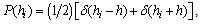(2)

where h defines the disorder (field) strength. Our effort benefitsfrom (i) the existence of robust computational methods of graphtheory at and (ii) the work of Hartmann andNowak[15] that have suggested accurate estimates ofthe critical field and the correlation length's exponent of the bimodal RFIM using theseground–statecalculations and linear sizes up to . Although Ref.[15] is the most thorough one in the literatureof the bimodal RFIM, we should note here that also other previousworks in the field have provided estimates for the set that compare well to these values[16,17].

2. Simulation at Zero Temperature

As it is well known, the random field is a relevant perturbationat the pure fixed point, and the random-field fixed point is at zero temperature[2]. We can therefore determine the critical behaviour, staying at and crossing the phase boundary at . This is a convenient approach because we candetermine the ground states exactly using efficient optimizationalgorithms[18-21] through an existing mapping of the ground state to the maximum– flowoptimization problem[22-24]. A clearadvantage of this approach is the ability to simulate large system sizes and disorder ensembles avoiding at the same time statisticalerrors and equilibration problems, which are the two majordrawbacks encountered in positive – temperature simulations of systems with rough free–energy landscapes [25]. The application of optimization algorithms to the RFIM is nowadays well established[25]. Here, we have implemented the Push–Relabelalgorithm of Goldberg and Tarjan[26], including also an interesting modification proposed by Middleton and Fisher[4].

The algorithm starts by assigning an excess to each latticesite i, with. Residual capacity variables between neighbouring sites are initially set to J. A height variable is then assigned to each node via a global updatestep. In this global update, the value of at each site inthe set of negative excesssites is set to zero. Sites with have set to thelength of the shortest path, via edges with positive capacity from i to T. The ground state is found by successively rearranging the excesses , via push operations, and updating the heights, viarelabel operations. When no more pushes or relabels are possible, a final global update determines the ground state, sothat sites which are path connected by bonds with to T have , while those which are disconnected from T have .

A push operation moves excessfrom a site i to a lower height neighbour j, if possible, thatis, whenever ,, and . In a push,the working variables are modified according to, where. Push operations tend to move thepositive excess towards sites in T. When and nopush is possible, the site is relabelled, with increased to 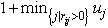. In addition, if a set ofhighest sites U becomes isolated, with , forall and all, the height forall is increased to its maximum value, N, asthese sites will always be isolated from the negative excessnodes. Periodic global updates are often crucial to the practicalspeed of the algorithm[4]. Following thesuggestions of Middleton and Fisher[4],we have also applied global updates here every N relabels, a practise found to be computationally optimum.Using this scheme, we performed simulations of the bimodal RFIMfor systems containing up to spins, for 5 candidate -values of the field strength in the range[2.18 - 2.22] with a step 0.01, following the proposed critical value of Ref.[15]. For each pair an extensive disorder averaging has beenundertaken by sampling over random– fieldrealizations.

3. Results and Discussion

In general, one expects that the finite – temperature definition of the specific heat C can be extended to zero temperature, with the second derivative of with respect to temperature being replaced by the second derivative of the ground–stateenergy density with respect to the random field h[4,12]. The first derivative is just

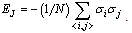(3)

The general finite – size scaling form assumed is that the singular part of the specific heatbehaves as

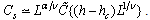(4)

Thus, one may estimate α by studying the behaviour of at [4]. The computation from the behaviour of is based on integrating Eq. (4) up to , which gives a dependence of the form

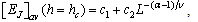(5)

with constants. Alternatively, following the prescription of Ref.[12], one may calculate the second derivative by finite differences of for values of h near and determine α by fitting to the maximum of the peaks in, which occur at . However, this latter approach may be more strongly affected by strong finite – size corrections, since the peaks in found by numerical differentiation are somewhat above , and furthermore is computationally more demanding since one must have the values of in a wide range of hvalues. In the present case, where the critical value is known with good accuracy[15], the first approach seems to be more suitable to follow.

Thus, using our numerical data we have constructed the disorder – averaged curves shown in Fig. 1 for all 5 values of the candidate critical field , as also indicated in the figure. The error bars shown reflect the sample – to – samplefluctuations in the ensemble of the disorder realizations. The solid lines are power – lawfittings of the form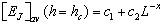, where. The estimates for the exponent x are also shown in Figure 1, each one next to the corresponding curve. Using now the estimate of Ref.[15] and the relation we calculate the critical exponent α of the specific heat and its error bars and we plot its dependence on in Fig. 2. Note that the rather large error bars come mainly from the error of the critical exponent ν used . The dotted line in this figure is a guide for the eye and marks the case . From Fig. 2 it is clear that the critical exponent α is very close to zero (especially for the value that has been proposed as the exact critical disorder strength of the bimodal RFIM we get . All this set of α–valuesis in accordance with the experimental prediction of a diverging specific heat[8] and also with the most extensive numerical works on the Gaussian RFIM that have predicted [4] and [14] using similar techniques.

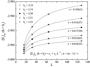Figure 1. Finite – size scaling behaviour of the bond part of the energy density at the 5 candidate values of the critical random – fieldstrength

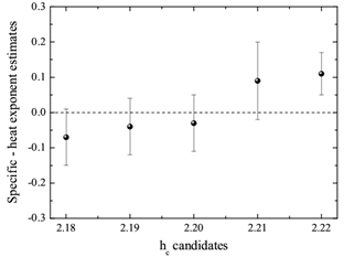Figure 2. Specific – heat exponent estimates as a function of the 5 candidate values for the critical field

4. Conclusions

In summary, we have presented an independent estimation of the critical exponent α of the bimodal RFIM. The scaling behaviour of the bond part of the energy density at the critical field indicated that, thus pointing at a logarithmic divergence of the specific heat, in agreement with experimental data[8], and also in agreement with the most important studies of the corresponding Gaussian model[4,14]. Our effort became feasible through the implementation of a modified version of the Push – Relabelalgorithm[4] that enabled us to simulate very large system sizes, up to spins, and disorder ensembles of the order of , for several values of the field strength. Clearly, such a computational task goes beyond the limits of any kind of positive – temperatureMonte Carlo scheme.

ACKNOWLEDGEMENTS

P.E.T. is grateful for financial support by the Austrian Science Foundation within the SFB ViCoM (Grant F41). I.G. acknowledges financial support by Marie Curie ITN-COMPLOIDS (Grant Agreement No. 234810). N.G.F. has been partly supported by MICINN, Spain, through Research Contract No. FIS2009-12648-C03.