Alhassan Shuaibu , M. Y. Onimisi
Department of Physics Nigerian Defence Academy, P.M.B.2019, Kaduna,Nigeria
Correspondence to: M. Y. Onimisi , Department of Physics Nigerian Defence Academy, P.M.B.2019, Kaduna,Nigeria.
| Email: |  |
Copyright © 2012 Scientific & Academic Publishing. All Rights Reserved.
Abstract
Results of theoretical models for calculations of electron energy levels in one-dimensional periodic potentials are presented. An appropriate equation to obtain the energy levels for electron subjected to any periodic potential such as Rectangular potential, Cosine potential, saw-toothed potentials is derived. An electron subjected to a rectangular potential under some limited parameters is considered. The computed values were obtained using the simulated Fortran Codes and ran on a FORTRAN 97 compiler o an accuracy of at least 1 percent. The results have shown good degree of accuracy when compared with the similar results in the some theoretical models.
Keywords:
One Dimensional Periodic Potentials, Nearly Free Approximation, Semiconductor, Schrödinger Equation
1.0 Introduction
A particular demanding area encountered in any solid state physics is that of obtaining the energies of electrons in crystals[2]. Familiarity with this work is the basis for proper understanding of electrical phenomena in metals and semiconductors; perhaps the most significant difficulty that arises is that any realistic treatment necessitates the use of numerical methods. Commonly, however only qualitative arguments or rather unrealistic models[1], such as the Kronig-Penney model which can be described analytically.Any system involving particles will exhibit quantum mechanical features if the de-Broglie wave length associated with the momentum of the particles is of the same order of magnitude or greater than a typical length over which the potential acting on the particles changes significantly[2].One particular formidable powerful way of obtaining the energy levels and energy bands using a Quantum mechanical method is by solving Schrödinger equation. Schrödinger equation is a form of differential equation, and almost all the analytical solutions are done mathematically. However, in contemporary research almost all the mathematical manipulations to the solution of Schrödinger equation is done not analytically, but rather by computer using numerical methods. There are cogent reasons for this. The solution of any kind of differential equation constitutes an entire sub discipline of mathematics; unfortunately different potential can be substituted into the Schrödinger equation which can yield a different problem requiring a different solution.No single method suffices for all potentials. Moreover, for most physically realistic potentials, the Schrödinger equation cannot be solved in analytic form. This is particularly true of real three-dimensional systems, such as many electron atoms, for which the potential experienced by each electron is determined by the configuration of all the other electrons in the atom[5]. For these cases and even for the majority of one-dimensional potentials it has become customary to resort to numerical approximation method, employing a computer to do the repetitive calculation involved. In contrast to analytic methods, the computer solution procedure for one-dimensional potentials can be standardized. Many attempts using different method or computer programming language have been used to obtain the energy band in one-dimensional Schrödinger equation. In this work we use a FORTRAN 97 code to solve the required Schrödinger equation. The computer program presented here enables the user to investigate electron energies in a system where the form, magnitude and the period of the potentials can be specified by the user. Also the effective mass and probability density of the electrons can be computed. The result can be compared with those derived from approximate analytic treatments such as core state method, nearly free electron model for certain ranges of the parameters.
1.1 Basic Equation
The time-independent Schr dinger equation for an electron in one-dimensional is given as[4]
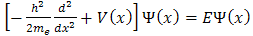 | (1) |
If we use the atomic units and measure energies in Rydberg’s and distance in A Bohr radius then this is equivalent to setting . Hence for electron equation (1) takes the form
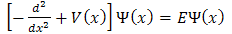 | (2) |
where V(x), the potential, is periodic with perioda, i.e.m is an integer. It might appear that  should also be periodic; in fact the reality is more complicated. The probability density
  is indeed Periodic with perioda, but this can still hold if
 is equal to the product of a function which is periodic and a complex conjugate is unity. The general form of such a complex quantity must be
 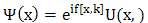 | (4) |
Substituting 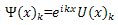 into equation (1) gives
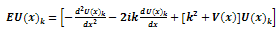 | (5) |
This is another form of Schrödinger equation and the solution to this form of the Schr dinger equation for the approximate potential V(x), has no exact analytic solutions[8], but numerical techniques can be used to achieve an accurate results.
1.2. The Nearly Free Electron Approximation
The opposite extreme of very low values of c can be treated using the nearly-free approximation[8]. If V(x) is small we can treat it as a perturbation and from the usual expression for non-degenerate perturbation theory, up to second order.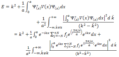 | (6) |
The factors  and
and  arise because the norm of the wave functions over the unit cell is a. the exponential functions are orthogonal over the unit cell,
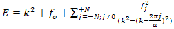 | (7) |
This equation is accurate except when there is degeneracy, or near degeneracy between the states at k and k- ,That is
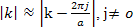 leading to k
 | (8) |
As will be the case in the region of the zone boundaries, we then need to consider the explicit form of the wave functions which in this case all the wave functions considered are periodic just as proposed by the Bloch theorem
1.3. The Effective Mass
There are situations, particularly those involving the dynamic behaviour of electrons, when the E-K relationship is not the most useful form in which to present the results of the band structure calculation. The wave functions in equation (5) extends over the entire space; if we want to represent the uniform motion of a localized electron the uncertainty principle indicates that we must build up a wave-packet with a spread of k-values[10]. The appropriate velocity is equal to the group velocity ( )which is equal to the derivative of the angular frequency (
 )with respect to k.
 | (9) |
E= since the reduced plank’s constant is unity in the atomic system of units.If a force F acts on this electron or wave-packet in the positive x direction then
 | (10) |
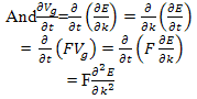 | (11) |
Comparing this result with the Newton’s second law of motion for a particle of mass M ,i.e. We can see that the motion of the electron wave-packet can be described by the semi-classical concept of an effective mass
 | (12) |
We should perhaps observe that there are situations[14] when a different definition of effective mass appears to be appropriate. | (13) |
For the lowest band  near k=0 but
  near
near  . Rather than refer to a negative mass it is conventional to take
  | (14) |
But to refer to electrons (with electron charge –e) when  and holes (with charge +e)- regarded as the absence of an electron from a band; for
 .It should be noted that since in the atomic system of units the mass of an electron
 ,
,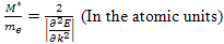 | (15) |
It is easy that this equation is plausible in the two extremes of completely free electrons and the core state approximation. For completely free electrons  and
and  . In this case of the core state approximation (where the electrons are not free to travel through the crystal) E is independent of k,
 | (16) |
If the nearly-free electron approximation apply then the approximate analytic expression for E(k) can be transformed to analytic expressions for  as a function of k.The seemingly perverse behaviour of holes can be understood if we recall that at the zone boundaries, Bragg reflection leads to wave functions which are standing wave[11]. Consequently, there are regions of the energy band approaching the zone boundaries where an increase in the energy leads to a decrease in the velocity- the acceleration is in the opposite direction of the force. The concept of holes is used to describe this unexpected behaviour.Having found the E at k=0,
  the program estimates
  at these k-values from the results for
  by Taylor’s series:
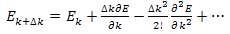 | (17) |
Hence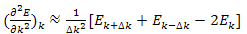 | (18) |
The program displays the results for  as function of k, printing a letter E (electron) when
  and a letter H (holes) for
  .
.
2. Results
We have run the program for rectangular potential based on equation 8. We have performed a series of runs varying chosen potentials while keeping the period constant. The first three energy levels are computed. The E-K relation and probability density are plotted.| Table 1. the first three energy levels for the Rectangular potential with a Height 5.0, Width 0.5 and period 1.5 |
| | K | E1(eV) | E2(eV) | E3(eV) | | 0.0000 | 1.4499 | 18.4804 | 20.0641 | | 0.1047 | 1.4603 | 18.1049 | 20.4621 | | 0.2094 | 1.4917 | 17.4000 | 21.2342 | | 0.3142 | 1.5440 | 16.6373 | 22.1089 | | 0.4189 | 1.6171 | 15.8717 | 23.0315 | | 0.5236 | 1.7109 | 15.1179 | 23.9872 | | 0.6283 | 1.8253 | 14.3814 | 24.9709 | | 0.7330 | 1.9600 | 13.6649 | 25.9800 | | 0.8378 | 2.1147 | 12.9698 | 27.0133 | | 0.9425 | 2.2890 | 12.2974 | 28.0700 | | 1.0472 | 2.4824 | 11.6486 | 29.1497 | | 1.1518 | 2.6940 | 11.0245 | 30.2533 | | 1.2566 | 2.9226 | 10.4265 | 31.3775 | | 1.3614 | 3.1666 | 9.8564 | 32.5252 | | 1.4761 | 3.4233 | 9.3169 | 33.6951 | | 1.5708 | 3.9548 | 8.8125 | 34.8874 | | 1.6755 | 3.9548 | 8.3501 | 36.1018 | | 1.7802 | 4.2107 | 7.9419 | 37.3383 | | 1.8850 | 4.4355 | 7.6082 | 38.5968 | | 1.9897 | 4.5970 | 7.3814 | 39.8768 | | 2.0944 | 4.6571 | 7.2995 | 41.1096 |
|
|
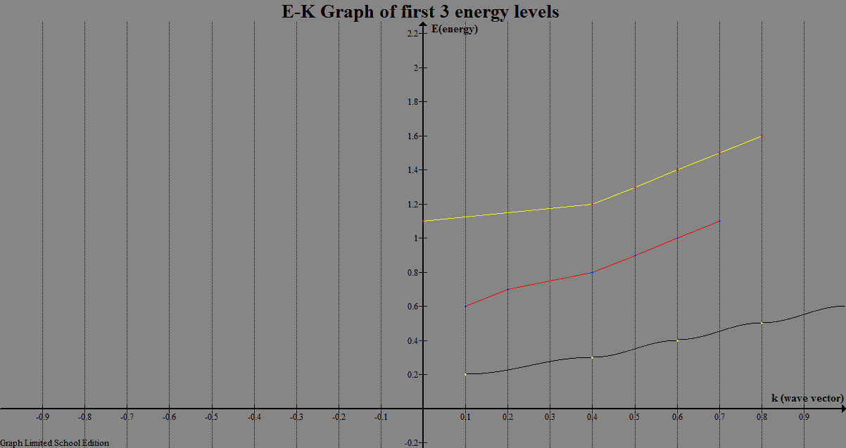 | Figure 1. E-K graph for the computed first 3 energy levels for Rectangular potential |
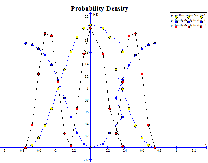 | Figure 2. Graph for probability density function for the first three energy levels |
3. Discussion
Having found the E at k=0, 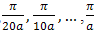 fig.(1.0) the program estimates
  at these k-values from the results for
  Hence
Hence The program also displays the results for
  as function of k, when
  and when
  .fig. (2.0)The simulated program can be used in a variety of ways and the accompanying documentation tailored to suit a variety of levels of user, but a particularly instructive procedure is to concentrate on one form of potential and first to perform a series of runs varying V0 over a wide range while keeping the period constant. It is then relatively simple for the cases of the rectangular potential, the cosine potential and the harmonic potential to compare graphically the energy difference between the first and second energy bands at
  (and or between the first, second and third bands at k=0) as a function of V0 with the predictions of the nearly-free electron approximation. In this way an estimate can be made of the value of V0 below which the nearly free electron approximation is accurate. A second criterion that aids in identifying which approximation, if any, is accurate is the form of the E-k relationship itself. If the energy gaps at the zone boundaries are small then the nearly-free electron approximation is likely to hold. The respective regions of validity and the extent of the intermediate region, more detailed comparisons involving the variation of E with k and the probability density can then be made.
4. Conclusions
It is recommended that the procedure described in this work first be used to identify the region of applicability of the free electron approximation; the region of validity of Free electron approximation extends to somewhat lower values of V0. In table 1.0 the data points show the results for a typical series of runs as suggested, employing the rectangular potential. From the graph it is clear that the nearly-free electron approximation is valid for the choice of the parameters employed. This conclusion is consistent with the variation of E with K and the form of the probability density found in that case.
References
| [1] | L. Pincherie, (1971): Electronic Energy Bands in Solids. Macdonald, London ISSBN 887-3245-88-7, PP 89-92. |
| [2] | R. de L., Kronnig and W. G.,(1931): Penny Proc Roy. Soc (London), AL30, 499. |
| [3] | A. P., French and E. F., Taylor, (1979): An Introduction to Quantum Physics, Chapman and Hall. ISBN 9971- 51-281-5,PP 345-362. |
| [4] | http://www.ecee.colorado.edu/~bart/book/book/chapter2/ch2_3.htm#2_3_4 |
| [5] | B. I., Tijjani (2002), A Guide to FOTRAN programming. Dept. of Physics Bayero University Kano,ISBN 978- 2149- 60-8,PP 5-11. |
| [6] | M.L., Cohen, V., Heine and D., Weaire (1970), Solid State Physics 24. |
| [7] | R. Barrei, International Conference on Material Science (1956) ,69 553. |
| [8] | Bratislava K., Nikolic,:Introduction to Solid State Physics, Department of Physics and Astronomy University of Delaware, USA, PHY 624 Lecture Note . |
| [9] | NAG – Numerical Algorithms Group (1999): Central Office, Oxford University Computing Laboratory, 13, Ban Bury Road, Oxford OX2 6NN, U.K |
| [10] | Charles Kettle (1996): An introduction to solid state physics 7th edition/1996 ISBN 0-471 11181-3 |
| [11] | C.S.,Gallinat, G.,Koblmuller, J.S. Brown, S. Bernard’s (2006): Speck. Appi.Phys.Lett.89, 032109 |
| [12] | K., Butcher and T., Tensely:Super Lattices Microstruct.38. 19 |
 Abstract
 Reference
 Full-Text PDF
 Full-Text HTML