1. Introduction

Mathematical disease models are important tools in analyzing the spread and the control of infectious diseases. These models are based on dividing the host population into compartments, each containing individuals that are identical in terms of their status with respect to the disease under consideration. For example, in the SIR model there are three compartments namely Susceptibles (S), Infections (I) and Removed (R). From the compartments, the set of equations will arise. The equations specify how the sizes of the compartment change overtime, and are linear and nonlinear. Solutions of these equations will yield, S(t) the size of susceptibles at time t, I(t) the size of infectious individuals at the time t, and R(t) the size of the removed population at a given time t. Solving nonlinear equations is more challenging than solving linear equations. Different authors use different methods to solve nonlinear equations.

In [1], Homotopy Analysis Method (HAM) was used to solve the differntial equations of the Susptible, Exposed, Infectious and Removed (SEIR) epidemic model. The results showed that the series solution converged very fast and the solutions were accurate. The Adomian Decomposition Method (ADM) was used to solve the mathematical model of malaria in [2]. The Laplace Adomian Decomposition Method (LADM) was applied to analyse the SEIR epidemic models of measles in [3]. In [4], the ADM was employed to solve the Human Immunodeficiency Virus (HIV) infection model of latently infected cells. In [5], the Laplace-Adomian decomposition method and the Homotopy perturbation techniques were used to obtain approximate solutions of the equation of the fractional dynamics of a corona virus mathematical model under a Caputo derivative.

The novel corona virus, also known as COVID-19, is a deadly disease which came into being in late 2019. It is believed to have originated from Wuhan city in China [6]. As of 23^rd May 2022, it had affected 227 countries with a total of 527, 804, 291 cases worldwide and 6,300,525 deaths [7]. Infected individuals present with fever, coughing, and sneezing as some of the symptoms. In severe cases, patients are diagnosed with pneumonia and shortness of breath. It is transmitted from human to human by inhaling droplets exhaled through normal breathing, coughing, and sneezing from infected persons [8]. Approximate incubation period is from 2-14 days from the time of contact. However, it may go up to 27 days. As for the asymptomatic individuals, they do not develop any symptoms and are not aware of their infection, yet they can transmit the disease, [9]. As a result, preventive measures such as lock-down policy, use of face masks in public places, washing of hands with soap, and using hand sanitizer were introduced in most affected countries.

This study focuses on the construction of a mathematical model to analyze the transmission dynamics of COVID-19 and solve it with modified Adomian decomposition method. The rest of the paper is organized as follows: in Section 2 we formulate the mathematical model of COVID-19 and analyze it. In section 3 we solve the mathematical model of COVID-19 using Adomain Decomposition Method (ADM) and Modified Adomian Decomposition Method (MADM). Section 4 presents the numerical analysis of the model and discussion. The conclusion comes in Section 5.

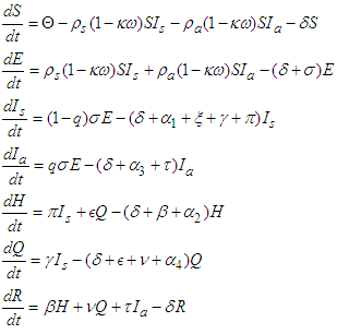
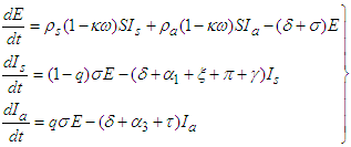
2. Model Formulation

The mathematical model of COVID-19 is developed by dividing the total population into seven classes. The variables Susceptible , Exposed , Symptomatic , Asymptomatic , Hospitalized , Quarantined and Recovered are used to represent the classes. Individuals are recruited into the susceptible class through the rate . The susceptible population is exposed to the disease through contact with symptomatic and asymptomatic infectious individuals. The parameters and represent the effective contact rates for individuals in the symptomatic and asymptomatic infectious classes, respectively. There is a fraction of individuals who use face masks in the population and it is given as , whereas represents the expected decrease in the risk of infection as a result of using face masks. The exposed individuals progress to infectious classes at the rate . A fraction of the exposed shows no symptoms and they proceed to asymptomatic infectious class whereas the remaining fraction shows symptoms of the disease and hence proceeds to the symptomatic class. The symptomatic infectious are hospitalized at the rate of and are quarantined at the rate of . The asymptomatic infectious recover at the rate . The quarantined are hospitalized at the rate and they recover at the rate whereas the hospitalized recover at the rate . There is a natural death rate of for individuals in all classes. 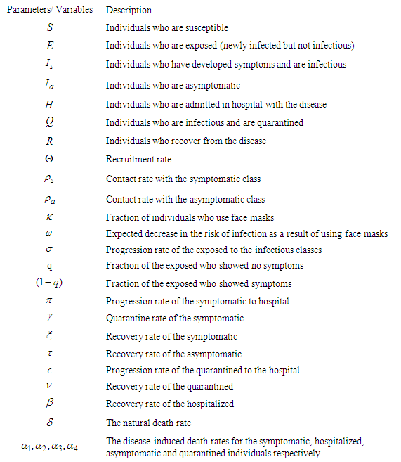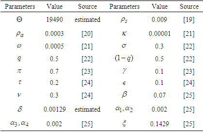Additionally, individuals in the symptomatic, hospitalized, asymptomatic, and quarantined classes have disease-induced death rates of , respectively. The summary of the description of the variables and parameters is given in Tables 1. Using the symbols and variables described in Table 1 we draw the compartmental model that shows the progression of the disease, given in Figure 1.

Table 1. Symbols and Description of Parameters

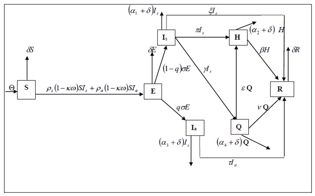Figure 1. Compartmental model of the transmission of COVID-19

Using the variables, parameters and the compartmental model we derive the system of ordinary differential model equations as follows:

(1)

The total population is given as,

(2)

and is given by

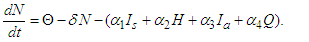(3)

2.1. Positivity and Boundedness of Solutions

2.1.1. Positivity of Solutions

Since the variables of model equation system (1) represent humans, it is important to show that they are positive.

Theorem 1 If the initial values are given by 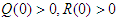then the solutions of the system equation (1) are positive for all .

Proof: Using the first equation of equation system (1), we have the following:

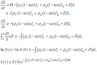Thus is positive since is positive and the exponential function 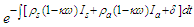is always positive. Using the same method, we can prove the rest of the equations of system equation (1) and show that

2.1.2. Boundedness of the Solutions

Theorem 2 All positive solutions presented in Theorem (1) are bounded.

Proof: In the absence of the disease, i.e , equation (3) becomes

which can be written as

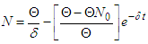, and as

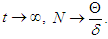Thus, we conclude that

(4)

Hence, the positive solutions of model equation (1) are bounded.

2.2. Existence and Stability of Equilibrium Points

The equilibrium points are calculated by equating the left hand side of equation system (1) to zero. This leads to the following system of equations,

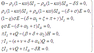(5)

2.2.1. The Disease Free Equilibrium Point (d_fep)

In the absence of infection 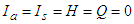. Solving the equations of system 5, we obtain .

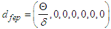2.2.2. The Reproduction Number of the Model

We compute the basic reproduction number R_C of the model system (1) by following [10]. The basic reproduction number measures the average number of new infections generated by a single infected person in a completely susceptible population.

Using the next generation matrix, we consider the classes that are actively transmitting the disease. These are:

(6)

Next, we find the matrices and which are the rate of appearance of new infections in compartment and transfer of individuals into and out of compartment by all other means, respectively. Here represents the infected classes, i. e 1, 2, 3. Thus we obtain,

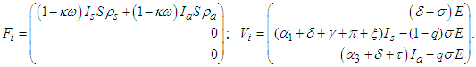Then taking partial derivatives of both and on the disease-free equilibrium point we get,

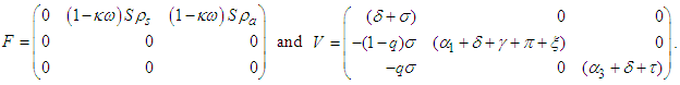Next we calculate the inverse of which is given by:

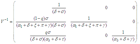The next generation matrix is given as the following product:

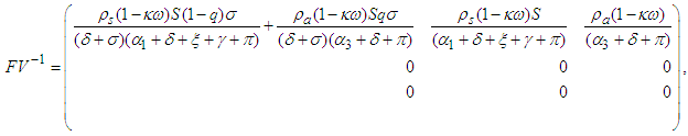and we calculate the eigenvalues of as follows:

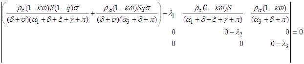Thus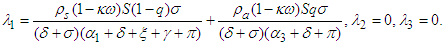

The reproduction number is given by the largest eigenvalue of the determinant of the matrix and so

(7)

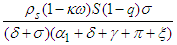Equation (7) consists of two reproduction numbers. The first reproduction number defines the number of new COVID-19 cases generated from the symptomatic infected individuals in class . The second reproduction number is 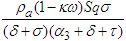which defines the number of new COVID-19 cases generated from the asymptomatic infectious individuals in class Hence the reproduction number is written as,

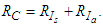(8)

2.2.3. Global Stability of the Disease-Free Equilibrium Point

The global stability of the disease-free equilibrium is established by the following theorem.

Theorem 3 If the disease-free equilibrium is globally asymptotically stable in and unstable if

We will use the Lyapunov function to show the stability of the disease-free equilibrium.

Let the Lyapunov function be

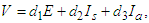(9)

where,

Let be the region that contains the origin. The we note that,

(i) ,

(ii) for all d1,d2,d3 since,

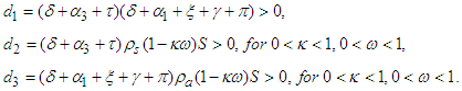Also and .

Thus we conclude that 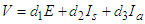is positive definite.

We now prove the stability of the disease-free equilibrium point using the Lyapunov function.

Proof: From equation (9), the derivative is given as

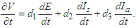(10)

But are given in equation system (1). Therefore,

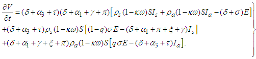(11)

The expansion of equation (11) yields,

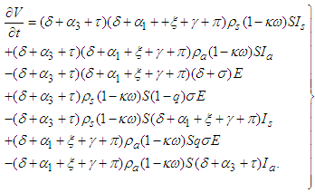(12)

Equation (12) can be simplified to

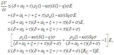Hence, if and if . By LaSalle's Invariance Principle [11], we conclude that the disease-free equilibrium of the model of COVID-19 is globally asymptotically stable in whenever

2.2.4. The Endemic Equilibrium Point

The endemic equilibrium point is denoted by 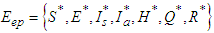and is calculated as,

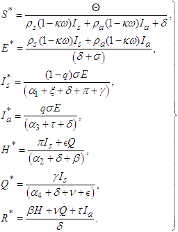(13)

2.2.5. Global Stability Analysis of the Endemic Equilibrium Point

The Lyapunov asymptotic stability theorem is used to prove the global asymptotic stability of the endemic equilibrium point. Using the method for constructing the Lyapunov function discussed in [12], we formulate the Lyapunov function for model equation (1).

Theorem 4 If , then the endemic equilibrium point of model equation (1) is globally asymptotically stable in the region

Proof First, we define Consider the function below:

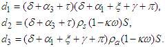
(14)

The derivative of along the solutions of the model in equation (1) is given by the expression:

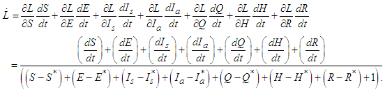(15)

From equation (4), all solutions of equation (13) satisfy the equality

(16)

In addition where, is the value that satisfies the condition . Thus Therefore,

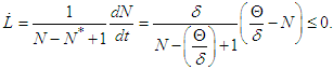
and are satisfied if and only if

is positive definite and is negative definite, hence the function is the Lyapunov function for model equation (1) and the endemic equilibrium is globally asymptotically stable by the Lyapunov asymptotic stability analysis [13]. Hence the proof.

3. Adomian Decomposition Method

In this section we apply the Adomian decomposition method proposed by George Adomian in the mid 1980's, [14] to solve the system equation (1).

3.1. Basic Concepts of the Adomian Decomposition Method

Let us consider the initial value problem expressed as

(17)

where is the linear operator, is the nonlinear operator and is the remaining linear part. By defining the inverse operator of as , we introduce it on both sides of equation (17) to get,

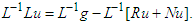(18)

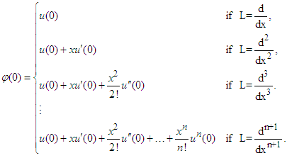
Solving for in equation (18) leads to,

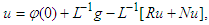(19)

where,

The Adomian Decomposition Method assumes that the unknown function can be expressed by an infinite series of the form,

(20)

where the component will be determined recursively. This method also defines the nonlinear term by the Adomian polynomials. More precisely, the ADM assumes that the nonlinear operator can be decomposed by an infinite series of polynomials given by,

(21)

where are the Adomian's polynomials defined as,

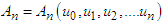(22)

and are calculated using the formular in [15]

(23)

Substituting equation (20) and equation (21) into equation (19) and using the fact that is a linear operator we obtain,

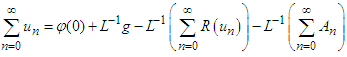(24)

Therefore the formal recurrence algorithm could be defined by,

(25)

The term approximation of the solution is given by,

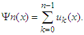(26)

The advantage of this method is that it solves problems in a direct way and in uncomplicated manner without linearization, perturbation or any unpreferable assumptions that may change the physical behaviour of the problem under discussion.

3.1.1. Solutions of the Mathematical Model of COVID-19 Using Adomian Decomposition Method

In order to explicitly construct approximate solutions of the system described by equation (1), we employ the Adomain decomposition method. To apply the Adomian decomposition method we choose: as initial approximations of Using equation (12) for calculating the Adomian polynomials for and as and respectively, we apply equation (24) to each of the equations in model system (1) to obtain the recursive algorithm for each equation as follows:

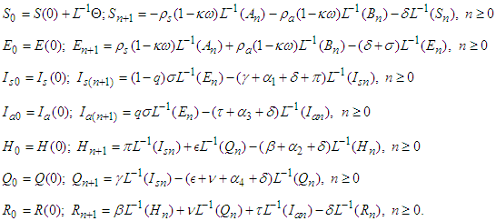Using equation (26) the solutons to equation (1) are obtained.

3.2. The Modified Adomian Decomposition Method

Here, we present the Modified Adomian Decomposition Method (MADM) which we use to solve the system of equations arising from the mathematical model of COVID-19. In [16], the authors proposed the modification of the ADM by introducing the terms 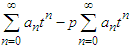into the calculations of the standard ADM. To understand the procedure of MADM we consider equation (23) and insert 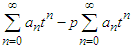to obtain:

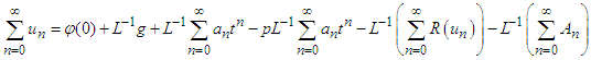(27)

So the recursive algorithm for MADM is defined as,

(28)

In this method we set and so that we solve for the coefficients for . The approximation of the solution is found by replacing the coefficients in the solution equation given by:

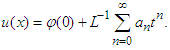(29)

The advantage of using MADM is that it reduces the computational size of the problem being solved because it involves the calculation of the first two iterations only. For nonlinear terms only the first Adomian polynomial is involved.

3.2.1. Solution of the Mathematical Model of COVID-19 using the Modified Adomian Decomposition Method

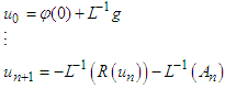
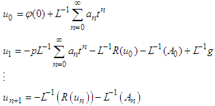
Applying equation (27) on each equation of system (1), we obtain the recursive relationship for each equation as follows:

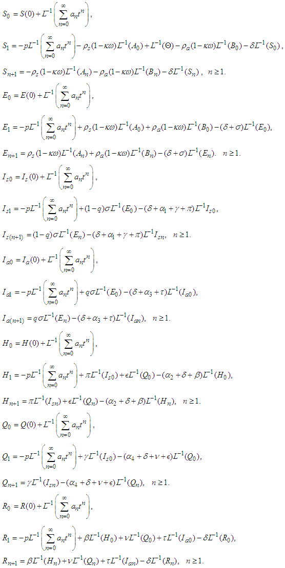Letting and setting we find the for . and replace in equation (29) to write the solution for equation system (1).

4. Results and Discussion

The results obtained from solving system equation (1) using ADM are compared with the results obtained using MADM.

We will use COVID -19 data for Zambia [17] as initial values and are given as . The natural death rate, is calculated by taking the reciprocal of the average life expectancy (in months). In Zambia the life expectancy is 64.70 years [18], hence 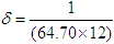. The population of Zambia is 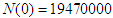[18]. Thus the recruitment is estimated as . The rest of the parameters are estimated from the literature as given in Table 2. Using the initial values and the parameter values we draw the graphs using SageMaths 9.0 software. The results are shown in Figure 2(a) to Figure 2(g).

Table 2. Parameter values

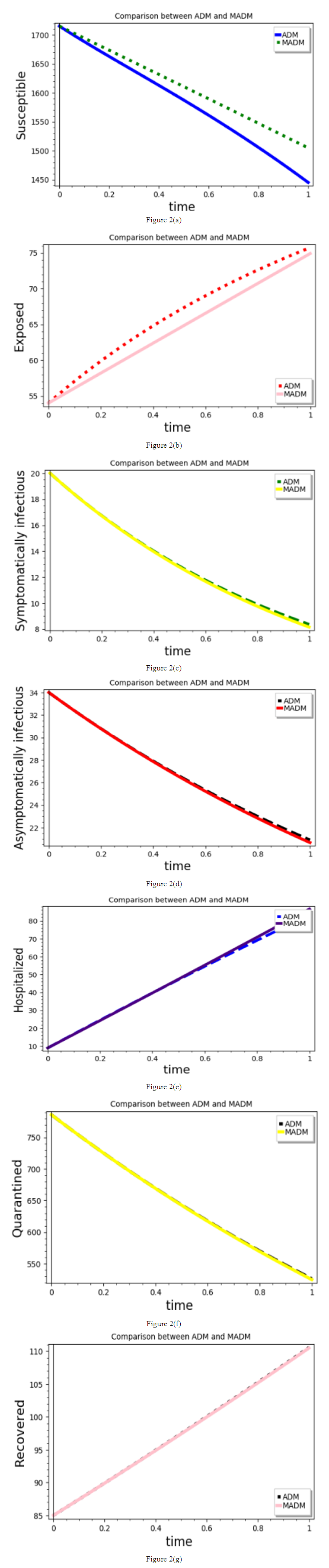Figure 2(a-g)

Figure 2(a) shows the results obtained by comparing MADM and ADM. MADM yields close solutions particularly for values of that are around zero. It is important to mention that for larger values of , the graphs are further away from each other.

In Figure 2(b), it is clearly seen that MADM and ADM solutions are in good agreement with each other for values of close to zero and one.

Figure 2(c), Figure 2(d), Figure 2(e), Figure 2(f) and Figure 2(g) indicate that MADM and ADM solutions are the same by coincidence.

The numerical analysis shown in the Figures above demonstrate the effectiveness of the modified Adomian decomposition method. The method gives highly accurate solutions with use of the first and second iterations only.

5. Conclusions

The model of COVID-19 has been formulated and its dynamical behaviour investigated. We showed that the population classes are non-negative. Using the next generation matrix, we calculated the basic reproduction number, R_C, which is useful in guiding control strategies. By constructing Lyapunov functions, we proved global stability of disease free and endemic equilibrium points. If the basic reproduction number is less 1, all solutions converge to the disease free equilibrium point and the disease dies out from the population. When the basic reproduction number is greater than 1, the endemic equilibruim point is globally stable, meaning that the disease will persist and the number of infected individuals tends to a positive constant. Lastly, it is well known that analytical solutions of nonlinear ordinary differential equations are difficult to find. In this paper, we solved nonlinear and linear Ordinary Differential Equations (ODEs) using ADM and MADM. It can be seen from numerical solutions in Fiqure 2 that we demonstrated the ability of ADM and MADM in solving ODEs. The series solutions converge very rapidly and from the graphs in Figure 2(a) to Figure 2(g), we can conclude that the ADM and MADM are very efficient and accurate methods in solving nonlinear mathematical models.

Data Availability: The data used to support the findings of this study is indicated within the article.

Conflict of interest: No potential conflict was reported by the authors.

Funding: This research did not receive any specific grant from funding agencies in the public, commercial or not-for-profit sectors.