M. Hameed, S. Boebel
Division of Mathematics & Computer Science, University of South Carolina, Spartanburg, SC, USA
Correspondence to: M. Hameed, Division of Mathematics & Computer Science, University of South Carolina, Spartanburg, SC, USA.
| Email: |  |
Copyright © 2023 The Author(s). Published by Scientific & Academic Publishing.
This work is licensed under the Creative Commons Attribution International License (CC BY).
http://creativecommons.org/licenses/by/4.0/

Abstract
In this work, we study of the laminar flow of a viscous Newtonian, conducting fluid confined between two stationary nonconducting porous disks, all under the influence of a transverse magnetic field of uniform intensity. Both disks are characterized by their porosity and are subject to constant fluid extraction or injection. To derive the governing equation for this flow, we use similarity transformation that reduces the Navier-Stokes equations to a single fourth order nonlinear equation that describes the flow field. Our solution strategy combines both analytical and numerical techniques. This integrated approach not only reinforces the methodological robustness of the study but also provides deeper insights into the underlying fluid dynamics. We present a detailed analysis of the impact of porosity and magnetic field on the flow profiles and supplements this with graphical representations of velocity profiles for different values of extraction and injection velocities.
Keywords:
Viscous flow, Porous disks, Magnetic field, Adomian Method
Cite this paper: M. Hameed, S. Boebel, Hybrid Adomian Method for MHD Viscous Flow Between Stationary Porous Disks, American Journal of Computational and Applied Mathematics , Vol. 13 No. 3, 2023, pp. 51-57. doi: 10.5923/j.ajcam.20231303.01.
1. Introduction
The investigation of fluid flow between two disks, a configuration frequently encountered in diverse industrial applications, including lubrication systems, in the design of thrust bearing, radial diffusers and geological fluid dynamics has long been a subject of extensive research. In this scenario, the presence of a porous medium, typically found in bearings, filters, and heat exchangers, adds an additional layer of complexity. Understanding and quantifying the fluid behaviour in this context are essential for optimizing the performance and longevity of such devices. A comprehensive understanding of viscous radial flow in porous media between stationary disks is critical for designing efficient and reliable engineering systems. The earlier work on this topic can be traced back to the pioneering work of Elkouh [1], in which he studied flows involving low Reynolds numbers associated with fluid extraction or injection at the disks. In a subsequent research endeavour, Elkouh [2] advanced our knowledge by providing perturbation solutions for cases where uniform injection or extraction velocities were applied at the disks. Numerous additional studies have delved into different facets of this problem. For example, in Rasmussen's work [3], the investigation focused on the steady viscous flow between porous disks, particularly in the context of mass suction. Rasmussen analysed the challenge of achieving a consistent flow of viscous fluid between two porous disks, aiming for equilibrium by incorporating equal injection or suction at both disks. Terrill and Cornish [4] investigated the radial flow between two uniformly porous disks using power series solution methods. In this thorough benchmark study, they considered many interesting physical aspects of the problem, studying the effect of both small as well as large suction or injection at the walls. Elcrat [5] further contributed to the work of Terrill and Cornish, and received recognition for his pioneering work in which he proved the existence of solutions and studied distinctive characteristics of viscous flow between two stationary porous disks, involving arbitrary uniform injection or suction.The presence of a magnetic field in this flow configuration introduces a fascinating dimension to the problem. Magnetic fields are known to exert a profound influence on the behaviour of fluids, particularly when the fluid has charged particles. This effect, often referred to as magnetohydrodynamics (MHD), has significant implications for a wide range of applications. The interaction of magnetic fields with fluid flows has been the subject of numerous studies, especially in the context of astrophysics, nuclear fusion, and energy generation. However, the application of MHD principles to viscous radial flow between porous disks remains relatively an underexplored and highly promising area of theoretical research.Chandrasekhara and Rudriah [6] conducted a comprehensive examination of continuous two-dimensional flow, where an incompressible conducting viscous fluid circulates between two parallel disks under the influence of a transverse magnetic field. They used perturbation techniques tailored for highly viscous creeping flow to derive a solution. However, it's important to note that this solution is only applicable to scenarios characterized by low suction or injection Reynolds numbers. In their subsequent work [7], they presented the analysis of three-dimensional axisymmetric flow between a rotating porous disk and a stationary porous disk. Their investigation considered parameters associated with both rotation and magnetic fields. This particular study was centred on the flow of a conducting fluid within the gap between two nonconducting disks, where one disk remained stationary while the other underwent rotation. They probed the effects of uniform suction or injection on velocity distribution and yielded asymptotic solutions. Notably, their findings indicated that uniform suction or injection exerted a significant influence on all velocity components, with the most pronounced impact observed on the radial velocity component, which predominated over the rotational effects. A few recent studies have attempted a numerical approach to explore the intricacies of viscous and viscoelastic radial flow when influenced by a magnetic field. Takhar et al. [8], for instance, employed finite element methods to solve equation for fluid flow and heat transfer with a micropolar fluid situated between two porous disks. In a parallel line of investigation, Bhat and Katagi [9] opted for a finite difference, Keller-Box approach to tackle the coupled nonlinear differential equations, ultimately yielding outcomes consistent with the earlier findings. By building upon the foundations laid by the aforementioned studies, this paper explores the complex interplay between viscous radial flow, porous media, and magnetic field, addressing the modelling, solution, underlying physics, and potential applications. We examine the flow of a conducting fluid in the gap between two stationary porous disks. Due to the geometry of the flow, it is assumed that normal fluid velocities are constant and flow in the axial direction is uniform. Under these conditions, we seek solutions having the property that the axial flow is uniform over the planes parallel to disks. Using a suitable similarity transformation, the Navier-Stokes equations are reduced to a fourth order nonlinear differential equation for axial velocity 𝑤. To solve this governing equation, we follow a non-traditional approach and introduce a new method, using a hybrid analytical-numerical approach based on Adomian Decomposition Method (ADM) and multivariate Newton-Raphson’s method. The Adomian Decomposition Method (ADM), introduced by George Adomian [10], has found widespread application in the solution of Initial Value Problems (IVPs) and Boundary Value Problems (BVPs) involving nonlinear ordinary or partial differential equations, integral equations, and integro-differential equations. One of its notable advantages is its ability to provide approximate analytical solutions without resorting to linearization, perturbation methods, discretization, making assumptions about initial terms, or the often challenging task of determining Green's functions. Researchers [11,12,13] have successfully harnessed the true capabilities of ADM as a valuable tool for investigating both analytical as well as numerical solutions to applied mathematics problems.
2. Mathematical Formulation
The flow geometry, as depicted in Figure 1, is characterized by its symmetry about a central axis perpendicular to both porous disks. In this context, we use cylindrical polar coordinates (𝑟, 𝜃, 𝑧), where 𝑟 represents the radial distance from the central axis, 𝜃 denotes the polar angle, and 𝑧 signifies the axial separation between the disks. The velocity components along the directions of increasing 𝑟 and 𝑧 are denoted by 𝑢 and 𝑤 respectively. The planes defined by 𝑧 = −𝐿, and 𝑧 = 𝐿 correspond to the planes of the infinite disks, establishing a channel of width 2𝐿. Within these porous disks, the fluid is either injected or extracted in a direction normal to the disks maintaining a constant velocity 𝑉1 at 𝑧 = −𝐿 and 𝑉2 at 𝑧 = 𝐿. It is essential to note that velocities may assume either positive or negative values, but for consistency, they are treated as positive in the positive 𝑧 direction. 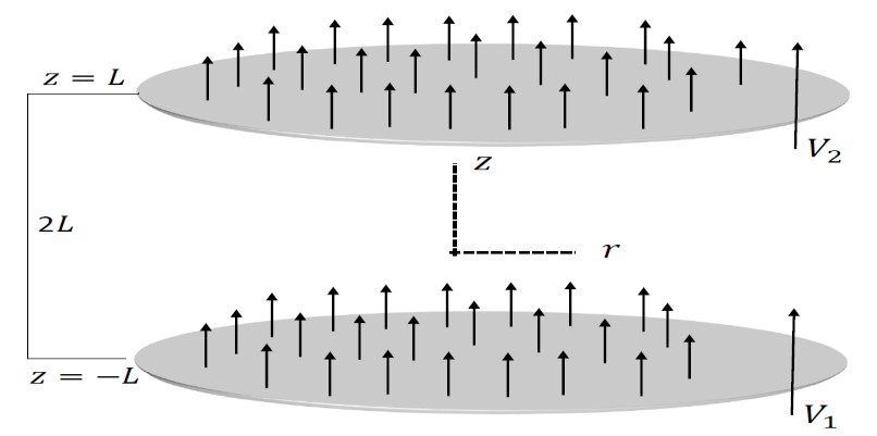 | Figure 1. Geometry of the flow between two porous disks |
We consider a steady, viscous incompressible, and conducting Newtonian fluid The Navier-Stokes equations for axisymmetric flow are: 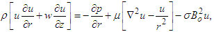 | (1) |
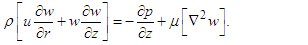 | (2) |
The continuity equation for incompressible fluid is given by: 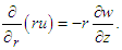 | (3) |
Here 𝑢 and 𝑤 represent the radial and axial components of the fluid velocity, 𝜌 and 𝜇 denote density and dynamic viscosity, 𝑝 is the kinematic pressure, and the Laplace operator  is defined as:
 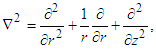 The boundary conditions at each disk are
 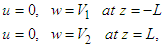 | (4) |
where 𝑉1 and 𝑉2 represent the constant velocities at which the fluid is injected or extracted normal to the disks.
3. Governing Equations
In this section, we outline the derivation of the govern-ing equation. We initiate this process by commencing with the classical Navier-Stokes equations. Utilizing the inherent symmetry of the flow, we proceed to derive a single govern-ing equation. It is important to note that, in our specific flow configuration, the axial velocity component 'w' represents the velocity perpendicular to the disks, which corresponds to the direction between the top and bottom disks. In this context, the flow maintains uniformity across planes that run parallel to the disks. Consequently, the velocity in the axial direction is exclusively a function of the axial coordinate 𝑧 and exhibits no dependency on the radial coordinate 𝑟. This phenomenon arises from the fact that the disks remain stationary, resulting in a consistent axial velocity as fluid moves radially from the centre to the outer region. This mathematical relationship can be expressed as follows:  | (5) |
With this information, we integrate continuity equation (3) with respect to 𝑟, to obtain: 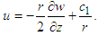 | (6) |
Here  is a constant of integration, chosen as zero, to en-sure finite velocity at 𝑟=0, simplifying equation (6) to
 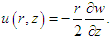 | (7) |
The velocity component 𝑢 is the velocity in the radial direction, i.e., towards or away from the center of the disks. The radial velocity can vary both with the radial coordinate 𝑟 and the axial coordinate 𝑧. It varies in the radial direction because the fluid is moving in and out from the center due to the radial flow. Therefore, 𝑢 = 𝑢(𝑟,𝑧).By substituting the velocity components w and u from Eq. (5, 7) into Eq. (1) & (2), the following equations are obtained: 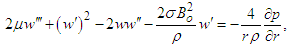 | (8) |
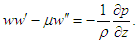 | (9) |
By differentiating Eq. (8) with respect to 𝑧 and Eq. (9) with respect to 𝑟, the following results are obtained: 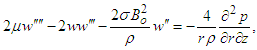 | (10) |
 | (11) |
Substituting Eq. (11) into Eq. (10), a single fourth-order nonlinear differential equation is derived: 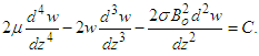 | (12) |
Moreover, it is evident from Eq. (11) that the pressure field must satisfy the following relation:  | (13) |
The non-dimensionalization of Eq. (12) is performed by introducing a new variable  and
and  After this transformation, the non-dimensional equation takes the form (after removing bars):
 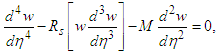 | (14) |
where  is the suction Reynolds number, and
 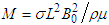 .Corresponding nondimensional boundary conditions at the disks take the form:
 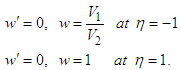 | (15) |
4. Solution Technique
We solve the fourth order nonlinear ordinary differential equation derived in the previous section using Hybrid Adomian Decomposition Method. This method relies on decomposing complex nonlinear equations into a series of simpler linear and nonlinear subproblems. It is particularly well-suited for nonlinear differential equations, offering an analytical approach that can provide accurate solutions without the need for traditional linearization techniques. To apply the Adomian decomposition method, we proceed with the governing equation given in (14), and write it in operator form:  | (16) |
Where, the L is the linear fourth order differential operator 𝐿=𝑑4/𝑑𝜂4 and we assume that the operator L is inverti-ble. Intuitively, our inverse operator is expressed in terms of four integrations with respect to 𝜂:  | (17) |
The symbol N in equation (16), represents the remaining nonlinear and linear terms as given in the following expres-sion  | (18) |
Apply the inverse operator 𝐿−1 to both sides of the Eq. (16) and arrive at  | (19) |
where 𝑁(𝑤)=𝑅𝑠𝑤𝑤′′′+𝑀𝑤′′, and 𝛼, 𝛽, 𝛾, and 𝛿 are arbitrary constants that result from the four integrations. These constants are unknown at this point, and will be determined subject to four boundary conditions as given in Eq. (15). In accordance with the established Adomian Decomposition method [11], we begin by breaking down the unknown function 𝑤 into an infinite series of components, as defined by the decomposition series:  | (20) |
The individual components, denoted as 𝑤𝑛 with n being greater than or equal to zero, can be efficiently computed through a recursive process. However, it is important to note that the nonlinear terms, represented as 𝑁(𝑤), must be ex-pressed in the form of an infinite series involving functions known as Adomian Polynomials:  | (21) |
To determine the Adomian polynomials 𝐴𝑛 for the nonlin-ear terms 𝑁(𝑤), a specific formula is employed [11]: 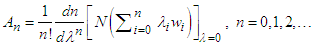 | (22) |
Here, λ serves as the grouping parameter. Few initial Adomian polynomials, derived using Equation (22), for a general nonlinear term 𝑁(𝑤) = 𝐹(𝑤), are given as follows: 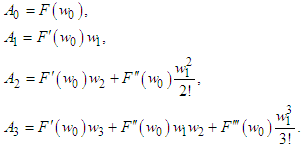 Substituting the series given in Eq. (20) & (21), in Eq. (19), we get
 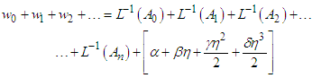 | (23) |
The zeroth component  is defined by all terms that are not included under the operator 𝐿−1. The remaining compo-nents can be computed recurrently such that each term is de-termined by using the previous components. Consequently, the components of 𝑤 can be elegantly determined using the recursive relations. Therefore,
 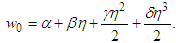 | (24) |
Then it follows from Eq. (22) by comparing both sides that  Hence, the Adomian approximate solution, denoted as
 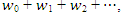 is dependent not only on η but also on the integration constants α, β, γ, and δ. In the conven-tional Adomian Decomposition Method (ADM) framework, these constants necessitate determination through a specified set of boundary conditions. However, the challenge arises as we lack essential information for this problem, specifically the boundary conditions for the unknown function and its first, second, and third derivatives. To address this constraint, we propose a novel hybrid approach that employs recurrence relations for calculating the coefficients of the Adomian polynomials. These coefficients are subsequently utilized in constructing the approximate solution 𝑤 through the assembly of the Adomian polynomials. To satisfy the given set of boundary conditions, we incorporate a numerical strategy by implementing the multivariate Newton's method. This entails the iterative determination of coefficient values for the Adomian polynomials, aligning them with the stipulated boundary conditions and thereby ensuring the satisfaction of these conditions by the approximate solution 𝑤. To implement this approach, we focus on the optimization of the integration constants 𝛼, 𝛽, 𝛾 and 𝛿 with the objective of fulfilling the prescribed boundary conditions:
 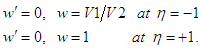 We form a set of equations incorporating the function 𝑤, which depends on the variables 𝛼, 𝛽, 𝛾, and 𝛿. This system ensures that at each boundary point, the boundary conditions are met. To accomplish this, we form a system of equations using
  such that at each boundary we get
 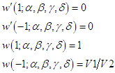 For the sake of simplicity, we introduce a vector
  .Consequently, system of equations can be succinctly rep-resented as follows:
 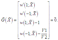 | (25) |
In order to solve the system  with four equations and four unknowns, we apply multivariate Newton-Raphson’s method. It is implemented as:
 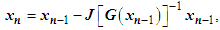 | (26) |
where  and
and  represents the Jacobian of 𝑮 evaluated at 𝒙𝑛−1. In our numerical calculations, we use a starting guess as
  which is a reasonable guess for a vector of constants, which optimizes the general solutions so that it satisfies the boundary conditions.
5. Numerical Solutions
In this section, we present numerical solutions obtained via our hybrid ADM approach. Initially, actual analytical solutions were derived using the standard Adomian method, incorporating four arbitrary constants (α, β, γ, and δ). Subsequently, these constants were optimized using the multivariate Newton's method while adhering to boundary conditions. Graphical results are shown for electrically conducting fluid flow between two infinitely large porous disks. The results demonstrate the influence of various fluid parameters, including extraction and injection velocities at the disks. Furthermore, the study assesses the impact of the magnetic field, characterized by parameter M, and examines how different combinations of suction and injection velocities (V1 and V2) affect the flow. To ensure the accuracy and reliability of our method, we validated the results against existing literature [4], particularly in cases without a magnetic field.
6. Concluding Remarks
This paper introduces a novel method for analyzing in-compressible viscous fluid flow between two porous disks in the presence of a transverse magnetic field. The proposed hybrid Adomian method combines analytical and numerical approaches, utilizing Adomian's method alongside Newton's Method to satisfy boundary conditions. Our results align well with established benchmark solutions in the absence of a magnetic field [5]. Numerical results are plotted that show the flow profile between two porous disks for four different physically relevant scenarios. Firgure-2 shows the plot of axial velocity 𝑤 in the case where fluid is injected at both disks. Injection here refers to the controlled introduction of a fluid into the flow system. It essentially creates a radial flow system, which influences the radial velocity distribution. The porous disks act as barriers through which the fluid must flow. As a result, the fluid distributes itself radially between the two disks. As observed from the figure 2, the higher the injection velocity 𝑽𝟏 the more fluid is forced to flow through that disk. Fluid injected with a positive velocity 𝑽𝟏 creates an outward radial flow from the first disk, conversely, the fluid injected with a negative velocity 𝑽𝟐 creates an inward radial flow towards the second disk, these two flows interact in the space between the two disks, and reach an equilibrium where the forces resulting from the injection velocities and pressure gradients balance out. 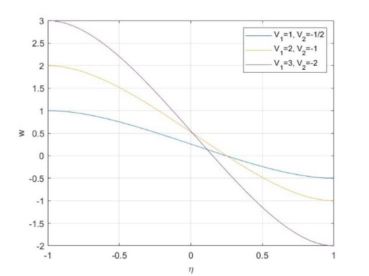 | Figure 2. Velocity 𝑤 in the case of injection at both disks (𝑉1>0, 𝑉2<0), and 𝑅𝑠=1, 𝑀=10 |
In Figure-3, we observe an intriguing scenario within the context of radial flow between two porous disks. This situa-tion involves the injection of fluid at one disk, denoted as 𝑉1>0, and extraction at the other disk, represented by 𝑉2≥0. Such a flow pattern leads to the development of a complex velocity distribution and the formation of a boundary layer. This configuration is commonly encountered in the engineering applications such as filtration systems. When fluid is injected from the first disk, it propagates radially outward, generating a velocity gradient as it approaches the extraction disk. The porous disks introduce resistance to the fluid flow, which, in turn, results in the formation of a boundary layer near the porous disk's surface. Within this boundary layer, the fluid's velocity experiences a significant reduction due to the interaction between the porous medium and the fluid. Figure-3 also illustrates an interesting case for 𝑉1=3 and 𝑉2=0, where the boundary layer assumes the characteristics of stagnation point flow, indicating that this particular boundary layer configuration is feasible when the normal velocity near the disk is directed towards this boundary. 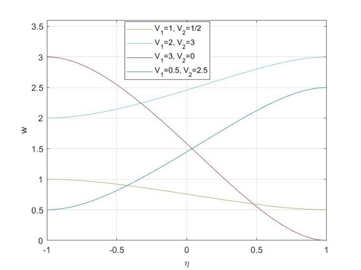 | Figure 3. Velocity 𝑤 in the case of extraction at one disks and injection at other (𝑉1>0, 𝑉2≥0) |
Figure-4 shows the results for the case when there is ex-traction at both porous disks (𝑉1<0, 𝑉2>0). It is noted that when we apply extraction at both disks, it tends to draw fluid radially inward from both disks. This inward flow de-creases the axial velocity near the boundary, creating a region of reduced axial velocity close to the disks.  | Figure 4. Velocity 𝑤 with extraction at both disks (𝑉1<0, 𝑉2>0), and 𝑅𝑠=10, 𝑀=10 |
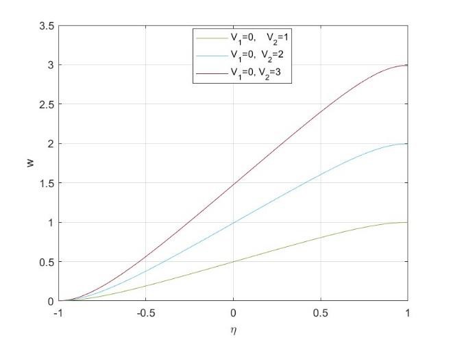 | Figure 5. Velocity 𝑤 in the case of transition between porosity at both disks (𝑉1=0, 𝑉2>0) |
Figures 6-7 depict the impact of the magnetic field on velocity. Increasing the magnetic field induces a complex and varied velocity field. Across a broad range of flow parameters, we observed a consistent decrease in velocity with an increasing Magnetic parameter M. Notably, dynamic changes occur near η=0.3, resulting in a reversal of flow direction. For the scenario where V1 > V2, velocity decreases with increasing M until just beyond the mid-plane. However, beyond η=0.3, this trend reverses, leading to an increase in velocity. Conversely, when V2 > V1, velocity rises with in-creasing M until η=0.3, after which it decreases. 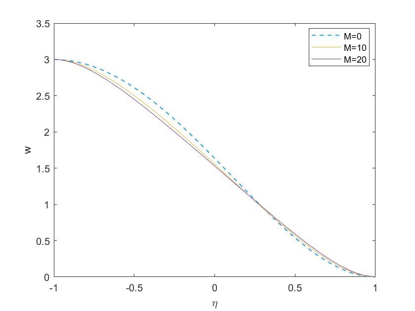 | Figure 6. Effect of magnetic field on the velocity 𝑤 with injection at both disks (𝑉1> 𝑉2) |
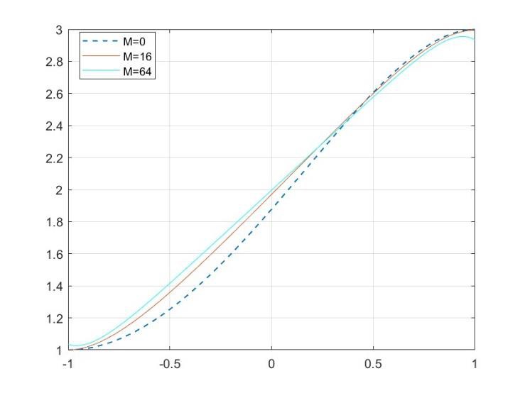 | Figure 7. Effect of magnetic field on velocity 𝑤 in for the case of (𝑉2> 𝑉1), and 𝑅𝑠=1 |
References
| [1] | A. Elkouh, “Laminar flow between porous disks,” Journal of the Engineering Mechanics Division., vol. 93(4) (1967), 31–38. |
| [2] | A. Elkouh, “Laminar source flow between parallel porous disks,” Appl. Sci. Res., vol. 21 (1969), pp. 284–302. |
| [3] | H. Rasmusseen, “Steady viscous flow between two porous disks,” Z. Angew. Math. Phys., vol. 21 (1970), 187–195. |
| [4] | R. Terrill, and J. Cornish, “Radial flow of a viscous, incom-pressible fluid between two stationary, unfirmly porous disks,” Journal of Applied Mathematics and Physics (ZAMP)., vol. 24(5) (1973), 676–688. |
| [5] | E. Elcrat, “Radial flow of a viscous fluid between porous disks,” Arch. Ration. Mech. Anal, vol. 61 (1976), 91–96. |
| [6] | B. Chandrasekhara, and N. Rudriah, “Magnetohydrodynamic laminar flow between porous disks,” Appl. Sci. Res, vol. 23 (1970), 42–52. |
| [7] | B. Chandrasekhara, and N. Rudriah, “Three dimensional MHD flow between porous disks,” Appl. Sci. Res, vol. 25 (1972), 179–192. |
| [8] | H. Takhar, R. Bhargava, R. Agrawal, and A. Balaji “ Finite element solutions of micropolar fluid flow and heat transfer between two porous disks,” International Journal of Engineering Science, vol. 38(2000), 1907-1922. |
| [9] | A. Bhat, and N. Katagi “ Micropolar fluid between nonpo-rous disk and a porous disk with slip: Keller-Box solution,” Ain Shams Engineering Journal, vol. 11(2020), 149-159. |
| [10] | G. Adomian, Solving Frontier problem of Physics: The De-composition Method, Kluwer Academic Press 1994. |
| [11] | A. M. Wazwaz, Partial Differential Equations, CRC Press 2002. |
| [12] | I. Hashim, M. Noorani, R. Ahmad, A. Bakar, E Ismail, and A. Zakaria, “Accuracy of the decomposition method applied to the Lorenz system,” Chaos, Solitons & Fractals, Vol. 28(2006), 1149-1158. |
| [13] | N. Sweilam, and M. Khader, “Approximate solutions to the nonlinear vibrations of the multiwalled carbon nanotubes using Adomian decomposition method,” Applied Mathematics and Computations, Vol. 217(2010), 495-505. |

 Abstract
 Reference
 Full-Text PDF
 Full-text HTML