Jonathan Ekow Quaicoe, Eric Neebo Wiah, Henry Otoo, Monica Veronica Crankson
Department of Mathematical Sciences, University of Mines and Technology, Tarkwa, Ghana
Correspondence to: Jonathan Ekow Quaicoe, Department of Mathematical Sciences, University of Mines and Technology, Tarkwa, Ghana.
| Email: |  |
Copyright © 2023 The Author(s). Published by Scientific & Academic Publishing.
This work is licensed under the Creative Commons Attribution International License (CC BY).
http://creativecommons.org/licenses/by/4.0/

Abstract
A deterministic control model of pollutants in tailings dam with the aim of reducing the pollutants in the wastewater is presented in this paper using a system of five ordinary differential equations. The qualitative analysis involves an assessment of the invariant region, the positivity of solutions, and the stability of equilibrium points. The next generation matrix was used to find the basic reproduction number  which was used as a threshold to determine the model's local and global stabilities. A sensitivity analysis was conducted to assess the influence of each model parameter in reducing pollutants in the wastewater. It was established that decreasing the parameters with negative sensitivity indices will help mitigate or eliminate pollutants in the tailings dam. This led to the application of optimal control theory to investigate the optimal strategy for reducing the pollutants in the tailings dam using a time-dependent control variable. The simulation result demonstrates the effects of the model parameters on each compartment in the model. This establishes that microbial flocculant is effective for reducing the concentration of pollutants in wastewater treatment processes.
Keywords:
Pollutants, Tailings dam, Goldmine wastewater, Microbial flocculants, Stability analysis, Optimal control
Cite this paper: Jonathan Ekow Quaicoe, Eric Neebo Wiah, Henry Otoo, Monica Veronica Crankson, Optimal Control Modelling of Gold Mine Wastewater Treatment in Tailings Dam, American Journal of Computational and Applied Mathematics , Vol. 13 No. 2, 2023, pp. 21-35. doi: 10.5923/j.ajcam.20231302.01.
1. Introduction
The mining industry generates tonnes of waste every year, including waste rock, tailings, and mine water [1]. Waste rock is generated from the extraction of ore from an open pit or underground mine and is usually deposited in heaps near the mine site [2]. Tailings and mine wastes are created during the processing of minerals, and water, which is a valuable resource in mining is used in most of the mining processes. While water is often recycled and reused, eventually it is collected and released into the environment along with the other wastes [3]. Tailings are typically pumped through pipes to be stored in a tailings’ storage facility, also known as the tailings dam or pond. The tailings dams have the potential for underground water pollution and a high risk of failure, which can result in the release of toxic heavy metals and cyanide-bearing solutions into the environment ([4], [5]). Wastewater from gold mines containing heavy metals and cyanide has become a major concern due to the risk it poses to humans and the environment [6]. The tailings dam where the wastewater is stored can potentially cause pollution if not properly treated. Various methods have been employed to remove heavy metals including physical, chemical, biological, or a combination of these methods [7]. However, most of these approaches are not environmentally friendly and economically feasible. In addition, heavy metals and cyanide are water-soluble, making it difficult to separate them through physical means. Physiochemical treatment techniques such as ion-exchange, reverse osmosis, ultrafiltration, dissolved air flotation, electrochemical precipitation, coagulation-flocculation, and electrodialysis have been used to remove heavy metals from wastewater, but there’s been some limitations in their applications due to high materials and operational costs. Furthermore, some of these techniques introduce secondary pollution, which requires further treatment [7]. Researchers have been exploring the use of microorganisms for heavy metal remediation and degradation as it is comparatively more effective, economical and environmentally friendly ([7], [8], [9]). Mathematical models have been developed for treating wastewater from the mining industries. A group of mathematical models describing microbial flocculants with nutrient competition and metabolic products in wastewater treatment was presented by [10]. The concept of continuous culture and fermentation were used to formulate the models. Their study showed how microbes compete for resources and produce different things as they grow. It was revealed that using microbial flocculants could help remove bad microbes from wastewater. A mathematical model was also developed to study the wastewater treatment process in an oxidation pond, specifically the effects of a biological-based product called mPHO on the degradation of contaminants and increase in dissolved oxygen levels [11]. They made use of a coupled system of ordinary differential equations to describe the correlation between the quantity of bacteria, chemical oxygen demand, and dissolved oxygen in the pond. The model was used to simulate the behavior of the system and the numerical results suggested a good approximation of the natural interaction processes between biological and chemical substances in the pond. A mathematical model on the microbial treatment of livestock and poultry sewage was also presented by [12]. The model examined the periodic addition of microbial flocculants for treating microorganisms like Escherichia coli in sewage. According to the findings, the system exhibited a microorganism's extinction periodic solution which is globally asymptotically stable when a certain threshold value is less than one, and the system is permanent when a certain threshold value is greater than one. An interesting experiment was conducted by [13] to investigate the kinetics and equilibrium of adsorption of heavy metals onto chitosan, which is a biopolymer obtained from crustacean shells. Chitosan is known to be capable of removing metallic ions from solutions and was thus utilized in wastewater treatment. The experiment involved studying the kinetic behavior of the adsorption process for various metallic ions at different concentrations and with different particle sizes in a batch system. The results revealed that the adsorption capacity of the chitosan is strongly dependent on the pH and specific metallic ions present in the solution. The study again showed that the particle size had a significant impact on the rate of metal uptake for each individual metallic ion.Despite attempts by researchers to reduce the pollutants in wastewater, optimal control theory for the treatment of goldmine wastewater in the tailings dam has not been proposed. This study therefore seeks to present an optimal control model for treating gold mine wastewater in tailings dams, with the goal of reducing pollutants in the wastewater. The study employs mathematical modelling to describe the kinetics of pollutant treatment in the tailings dam using microbial flocculants.
2. Model Description
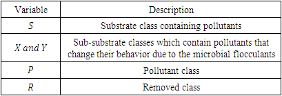
A deterministic control model with potential applications in utilizing microbial metabolites as flocculants for pollutant control in the Gold Mine tailings’ dam is proposed. The model comprises of the Substrate, Pollutant and Removed classes. The doses of microbial flocculants used as the control helps to change the behavior of some of the pollutants in the substrate. This change in behavior leads to subdividing the substrate into three subclasses, namely S, X and Y. A proportion of the substrate S with pollutants change their behavior due to the effect of the doses of microbial flocculants and thus, enter into the X and Y classes with different transmission rates. These X and Y classes will then have lower toxicity levels than the S class and will contribute to reduce the quantity of pollutants thereby resulting in the removal or reduction in the concentrations of pollutants in the tailings’ dam as seen in Figure 1. Only the dilution rate is taken into account with all other specific pollutant removal rates neglected. The substrate with pollutants is introduced into the tailings’ dam with a constant dilution rate  and an input concentration
  Since there are three substrate classes, three polluted rates
  are proposed for
  respectively for their interactions with the Polluted class,
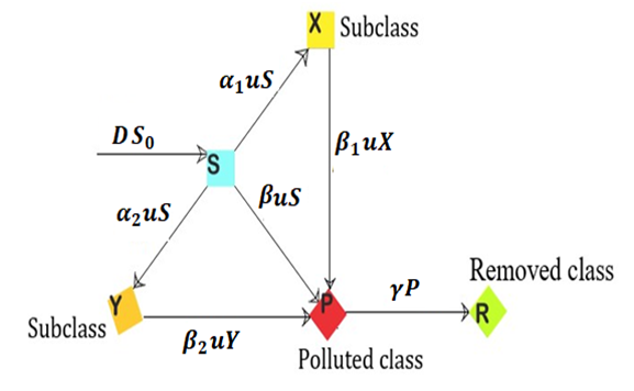 | Figure 1. A Schematic Flow Diagram of the Model |
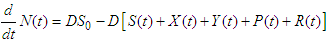
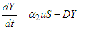
The deterministic control model comprising of a system of ordinary differential equations (ODEs) describing the rate of change of the various classes (S, X, Y, P and R) is given as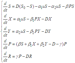 | (1) |
subject to the initial conditions;  .We note that
  is the entire population at time 𝑡.
Table 1. Description of the Model State Variables
 |
| |
|
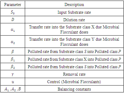
Table 2. Description of the Model Parameters
 |
| |
|
2.1. Model Assumptions
Ø The system is assumed to be well mixed to ensure uniformity in the concentration of the pollutants throughout the system.Ø The behavior of all the individual specific pollutant and their removal rates are neglected Ø Only substrate with pollutants is introduced into the tailings’ dam with a constant dilution rate DØ Factors like the pH, temperature and other environmental factors are kept constantØ All the parameters in the model are non-negative
3. The Model Analyses
In this section, the qualitative aspects of the model are explored. The concepts like the invariant region, positivity of the solution, equilibrium points, stability analysis, basic reproduction number, and sensitivity analysis are investigated.
3.1. The Invariant Region
Definition 3.1: A region in which the solutions to the model are uniformly bounded is defined as:  . The total population in the system is represented by
 | (2) |
which implies that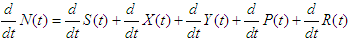 | (3) |
Substituting Equation (1) into Equation (3) yields;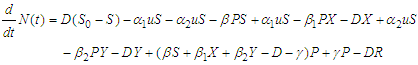 | (4) |
Evaluating yields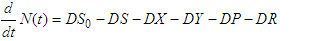 | (5) |
 | (6) |
Accordingly,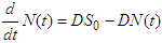 | (7) |
Integrating both sides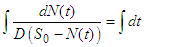 | (8) |
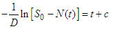 | (9) |
where c is a constant of integration. Thus,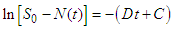 | (10) |
 | (11) |
 | (12) |
where  At
At  , let
, let  . This implies
 | (13) |
From Equations (12) and (13),  | (14) |
 | (15) |
As  Thus,
Thus, | (16) |
Hence, the feasible set of the solution of the model equations enter and remain in the invariant region: | (17) |
3.2. The Positivity of the Solution
The Positivity Theorem 3.2.Let then the solution (S, X, Y, P, R) are positive for
  .ProofConsidering the first equation of the model (1)
 | (18) |
 | (19) |
and accordingly, | (20) |
 | (21) |
 | (22) |
where | (23) |
and c represents the constant of integration. This implies that  | (24) |
 | (25) |
 | (26) |
where  .From the theorem, at
  This implies that
 | (27) |
Since  then
then | (28) |
Using the same approach on the remaining equations within the system, the second equation produces the following result: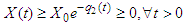 | (29) |
where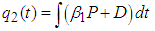 | (30) |
The third equation yields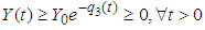 | (31) |
where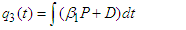 | (32) |
The fourth equation yields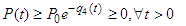 | (33) |
where 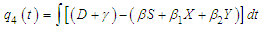 | (34) |
The fifth equation yields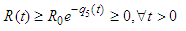 | (35) |
where 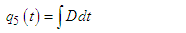 | (36) |
This completes the proof of the theorem.
3.3. The Pollutant Free Equilibrium State
In the developed model, we achieve a state where the pollutants are entirely absent. This state, referred to as a Pollutant Free Equilibrium (PFE), represents a solution where the population under study exists without exposure to the pollutants.The Model (1) has a pollutant free equilibrium obtained by setting the left-hand sides of the equations in the model (1) to zero, that is 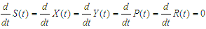 | (37) |
This yields the system of equations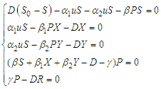 | (38) |
Solving the above system of equations results in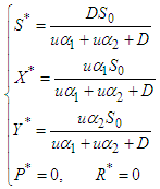 | (39) |
3.4. The Basic Reproduction Number 
In the concept of mathematical modelling,  stands as a fundamental threshold which aids in fully ascertaining the specific outcome of the system. The principle of the next generation matrix dictates that
  corresponds to the spectral radius of the model's next generation matrix
  .The
.The  associated with (1) is given as
 | (40) |
where
 signifies the rate at which fresh pollutants emerge within compartment
  , while
  denotes the influx of individuals into compartment
  .The matrix
  and
and  are obtained as,
 | (41) |
 | (42) |
It follows that the basic reproduction number of the model, denoted by  is
is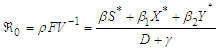 | (43) |
where  is the spectral radius.Substituting Equation (39) into Equation (43) results in
 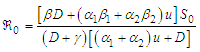 | (44) |
3.5. Stability Analyses
The equilibrium points of a system can be classified as stable, unstable, or asymptotically stable according to the nature of the eigenvalues of the coefficient matrix of the system of ODE or the Jacobian matrix of the nonlinear systems of ODE about such a point.
3.5.1. Local Stability
The local asymptotic stability of differential equations is established by applying the Routh-Hurwitz stability criterion which states that a system of ordinary differential equations is locally asymptotic stable at a particular point if all the eigenvalues of its Jacobian matrix are strictly negative or complex with negative real parts at that point.Theorem 3.5.1: The Pollutant Free Equilibrium PFE is Locally Asymptotically Stable LAS if  and unstable if
  .Lemma 3.5.1: The Pollutant Free Equilibrium PFE of the model in (1) is Locally Asymptotically Stable (LAS) if
  and unstable if
  .The Jacobian matrix J of the control model in (1) is given as
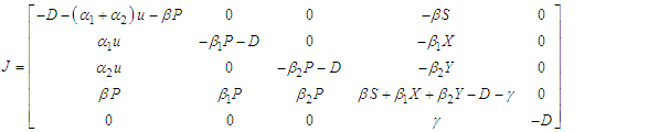 | (45) |
The Jacobian matrix J using equation (39) results in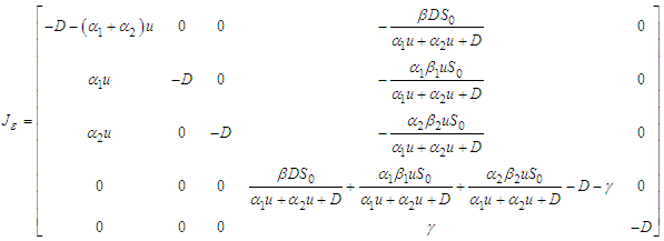 | (46) |
The eigenvalues of the Jacobian matrix,  is given as
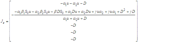 | (47) |
which implies that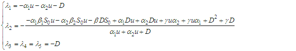 | (48) |
Clearly, all the eigenvalues of the Jacobian matrix are strictly negative, indicating that the model is locally asymptotically stable.
3.5.2. Global Stability of the Pollutant Free Equilibrium PFE
We examine the global asymptotic stability of the model in equation (1) using the methodology outlined by [15]. The model is denoted by: 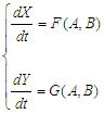 | (49) |
where  denotes the unpolluted population and
  denotes the polluted population.Theorem 3.5.2: The Pollutant Free Equilibrium is said to be Globally Asymptotically stable in
  if
if  and the following two conditions hold:C1: For
 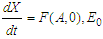 is globally asymptotically stable.C2:
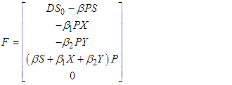
 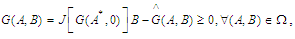 where,
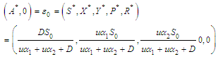 | (50) |
 is the Jacobian of
  obtained with respect to
  and evaluated at
  .ProofC1: From the control model (1), it follows that:
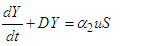
 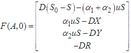 | (51) |
From the equation (51), it is clear that | (52) |
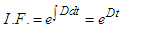
This can be confirmed through the application of the integrating factors technique.From the equation (51), we have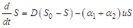 | (53) |
which can be written in standard form as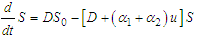 | (54) |
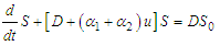 | (55) |
The integrating factor is given as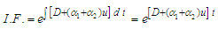 | (56) |
Multiplying equation (55) by (56) yields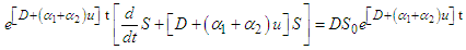 | (57) |
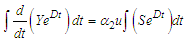
 | (58) |
 | (59) |
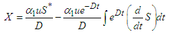
where C is a constant of integration. This implies | (60) |
As  ,
, | (61) |
From Equation (51), we also have | (62) |
 | (63) |
 | (64) |
Multiplying Equation (63) by (64) gives | (65) |
 | (66) |
 | (67) |
Using integration by parts to evaluate  gives
gives | (68) |
 | (69) |
Substituting Equation (69) into Equation (67) gives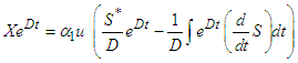 | (70) |
 | (71) |
As  ,
, | (72) |
Substituting Equation (61) into Equation (72) yields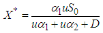 | (73) |
 | (74) |
 | (75) |
 | (76) |
Multiplying through Equation (75) by Equation (76) 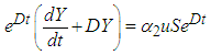 | (77) |
 | (78) |
 | (79) |
Substituting (69) into Equation (79) yields | (80) |
 | (81) |
As 
 | (82) |
Substituting Equation (61) into Equation (82) yields | (83) |
Accordingly, | (84) |
 | (85) |
 | (86) |
Multiply equation (85) by (86)  | (87) |
 | (88) |
 | (89) |
Hence C1 is satisfied.For C2:  | (91) |
 | (92) |
Clearly  , thus it follows from theorem (3.5.2) that PFE,
  is globally asymptotically stable.
3.6. Sensitivity Analysis
Performing sensitivity analysis is an important part of model validation. This step is necessary in this research study because it helps in assessing the impact of the parameters on the model results. Therefore, a sensitivity analysis is conducted to assess the model's resilience to parameter variations. Additionally, this analysis assists in identifying the parameters that exert the most substantial influence on  , offering insight into which parameters should be prioritized in the development of control strategies.Sensitivity indices quantify how a variable responds relative to changes in parameters. The normalized forward sensitivity index of
  concerning a parameter
  is calculated as the ratio of the relative change in
  to the relative change in the parameter
  . In cases where the variable is a differentiable function of the parameter, the sensitivity index can be formally defined as follows:Definition 3.6.1
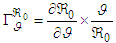 | (93) |
where
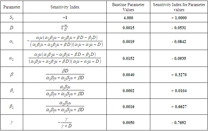
Table 3. Sensitivity Index of Each Model Parameter on

 |
| |
|
where  | (94) |
With the explicit formula provided in Equation (44) for  it is straightforward to derive an analytical expression for its sensitivity concerning each constituent parameter. The resultant values, as shown in Table 3, represent sensitivity indices for the default parameter values. It is worth noting that the sensitivity index (found in column 2 of Table 3) can vary in complexity based on the system's various parameters, but it may also manifest as a constant value, unrelated to any parameter. Column 4 of Table 3 provides these index values while considering the parameter values presented in column 3 of Table 3.A positive sensitivity index indicates a direct proportionality between the parameter and the value of
  . Consequently, a percentage increase in any of the parameters
  and
and  will result in an increase in
  , consequently raising the pollutant concentration within the tailings dam. Conversely, parameters exhibiting negative sensitivity indices signify an inverse relationship with
  . Thus, increasing the value of any of these parameters
  and
and  while keeping all other factors constant, will diminish
  . This, in turn, contributes to a reduction or elimination of the pollutants. For instance, increasing the value of the parameter
  by 10% will lead to a 3.27% increase on
  while increasing the value of the parameter
  by 10% will result in the reduction of 11.25% on
  . Parameters exhibiting high sensitivity demand meticulous estimation due to the fact that even slight variations in these parameters can yield substantial quantitative alterations. Conversely, insensitive parameters necessitate less rigorous estimation since minor fluctuations in such parameters have minimal impact on the quantity of interest.
4. Formulation and Analysis of the Optimal Control Problem
The use of suitable microbial flocculants as a time-dependent control  is bounded. The goal is to minimize the concentration of the pollutants, that is, the P class and to maximize the X and Y classes. These comprise of the pollutants in the S class and the pollutants changing behaviour as a result of the introduction of suitable microbial flocculants. Mathematically, for a fixed terminal time (T), the optimal control problem is to minimize the objective functional
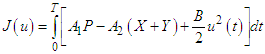 | (95) |
subject to the system of equation in (1) with appropriate state initial conditions.  and
and  are the positive relative weights of the pollutants and sub-substrates respectively. B is the positive relative weights of the control
  while
while  represents the cost control. T is the final time of control implementation. The Lebesgue measurable control set U is defined as
  where
where  is a measurable function such that
 . The goal of formulating the objective function is to find an optimal control
  such that
  | (96) |
4.1. Existence of an Optimal Control
This section presents the existence of an optimal control solution for the state system. This involves validating the sufficient conditions that guarantee the existence of a solution to the optimal control problem as stated in the following theorem obtained by [14]. The theorem is stated and proven with respect to the formulated optimal control problem.Theorem 4.1: Consider the optimal control problem (95) subject to the state equations (1) and initial conditions  There exists an optimal control
  with a corresponding solution set
  to the control model that minimizes
  over U if the following conditions are satisfied;Condition 1: The model equations, along with the initial conditions and the related control function in U, collectively constitute a non-empty set of solutions.Condition 2: The control set U is both closed and convex.Condition 3: The state system can be expressed as a linear function of the control variables, with coefficients that depend on both time and state variables.Condition 4: The Lagrangian
 of equation (95) is convex over U.Condition 5: There exist constants
  and
and  such that;
 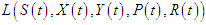 is bounded below by
  .In order to verify Condition 1, the model is written in the form:
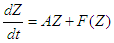 | (97) |
where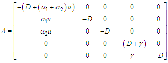 | (98) |
 | (99) |
 | (100) |
It is observed that the system (97) is non-linear with bounded coefficients. Thus, setting | (101) |
Then  in equation (101) satisfies
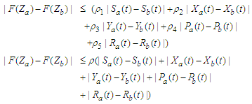 | (102) |
This implies that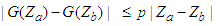 | (103) |
where 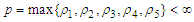 is a positive constant independent of the state variables and
 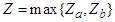 Consequently, as implied by equation (103), the function is uniformly Lipschitz continuous. Given the bounded nature of the control variables, it is evident that a solution to the model is viable, affirming the satisfaction of condition 1. Furthermore, the boundedness of the control set U conforms to its definition and since every bounded set is closed, then U is closed. Similarly, the set U is convex since
  , then any line joining any two points within the set will lie entirely within the set since the set is connected. Hence condition 2 holds.From the system of equations in (1), it is observed that the state equations depend on the control linearly, thus condition 3 is verified.Furthermore, since the Lagrangian is quadratic in the control and every quadratic function is convex, then it follows directly that the Lagrangian function of Equation (95) is convex. Thus, condition 4 is verified.Finally condition 5 is verified as follows;The Lagrangian function is defined as;
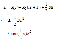 | (104) |
Since 
4.2. Necessary Condition of the Control
The primary approach for addressing an optimal control problem involves resolving a set of requisite conditions, which both the optimal control problem and its associated state(s) must comply to.This necessary condition was developed by Pontraygin in 1950. Pontraygin introduced the idea of adjoint functions to append the state system to the objective functional. This necessary condition, otherwise referred to as optimality condition, can be generated from the Hamilton function,  which is defined as follows;
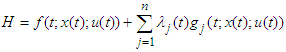 | (105) |
where  are the state equations.The Pontraygin’s Maximum Principle (PMP) converts the objective functional in equation (95) and the constraints in Equation (1) into a problem of pointwise minimization of a Hamiltonian, H with respect to
  . The Hamiltonian, H is defined as
 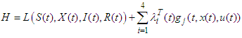 | (106) |
where  are the right-hand side of the five (5) state equations in (1),
  are the co-state or adjoint variables and
  , for
, for  . Hence
 | (107) |
Theorem 4.2: Pontryagin’s Maximum Principle theorem states that if  and
and  are optimal for problem (95), then there exist a piecewise differentiable adjoint variable
  such that
  and for all control(s)
  at each time
  , where the Hamiltonian, H is as defined in (107),
  (adjoint condition) with
  at
at  (optimality condition) and
  (transversality condition)
 | (108) |
 | (109) |
 | (110) |
 | (111) |
 | (112) |
 | (113) |
The adjoint system/conditions evaluated at the corresponding optimal solutions of the state equations are derived below; | (114) |
 | (115) |
 | (116) |
 | (117) |
 | (118) |
where | (119) |
are the transversality conditions.
4.3. Characterization of Optimal Controls
The optimal control  is characterized which provides the most favourable values for different control measures, along with their corresponding states
  .The Hamiltonian is minimized by taking the partial derivatives of
  with respect to the control
  . This gives the optimal solution to the Hamiltonian function. Thus,
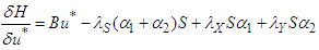 | (120) |
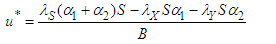
The optimality condition  is imposed on the equation above at
  . Therefore, the expression for the control variable
  is obtained as;
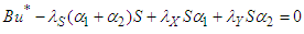 | (121) |
 | (122) |
Imposing the bound  on the control gives
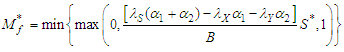 | (123) |
5. Results of Numerical Simulations
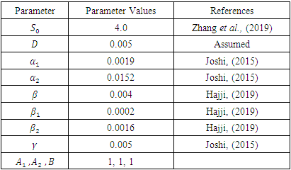
The numerical solutions of the resulting optimality system which comprises of the system of the model state equations and the corresponding adjoint equations with the optimal control characterization are presented. This was executed using MATLAB by employing the Forward-Backward Sweep method. The parameter values used for this numerical simulation are given in Table 4. All the positive relative weights of the Polluted and substrate classes in the simulations carried out here are only of theoretical sense to illustrate the control strategies. The analysis is done over a period of 60 days and the graphs and discussions of the results for the various control measures with their corresponding control profiles are also presented. This optimality system is solved with the following initial conditions: 
 With no control, the basic reproductive number
  thus, indicating the pollutant free equilibrium is unstable.
Table 4. Baseline Parameter Values
 |
| |
|
6. Discussions of the Numerical Results
Figure 2. gives the numerical simulation of each of the model compartment in a time span of 60 days. It shows a higher concentration of pollutants in substrate class, S in the absence of microbial flocculants (without control) as compared to the presence of the control. This is due to the fact that pollutants in the tailing’s dam are not changing their behavior to move to either of the two other substrate classes X and Y. 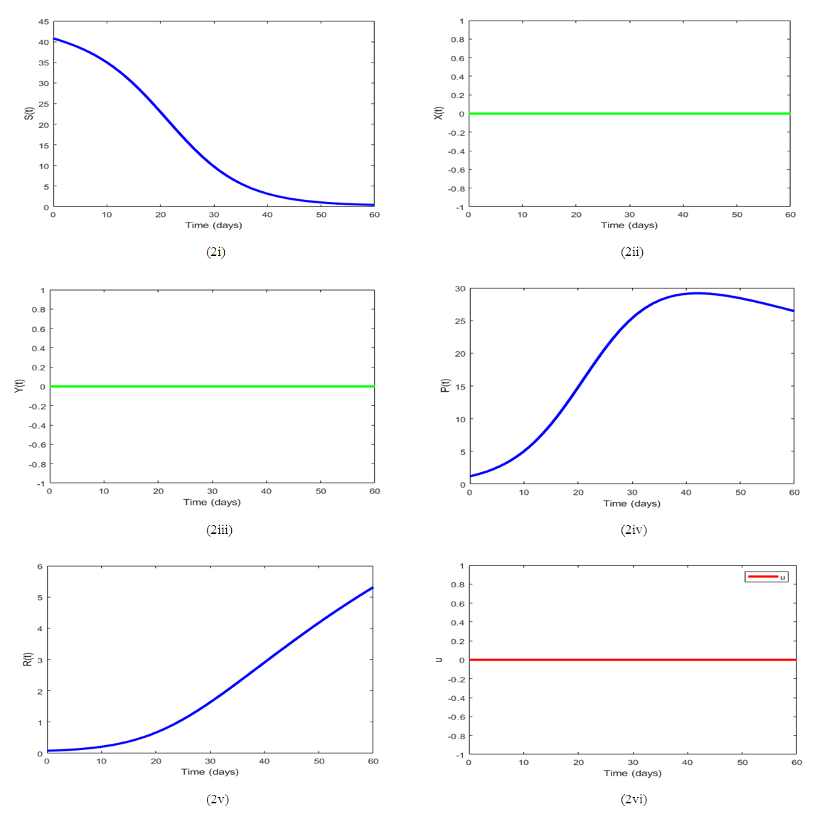 | Figure 2. Simulation results for (1), utilizing the default parameter values outlined in Table 3. and without a control |
Figure 3. shows that the substrate class, S decreases rapidly within the first 30 days due to the application of the control (microbial flocculant). The levels of the concentration of the pollutants in class P has decreased as compared to that of the Figure 1, demonstrating how effective the control can be. The control profile (u) of the Figure 2 demonstrates that to achieve an effective outcome, the control has to be applied at its upper bound for about 36 to 37 days. 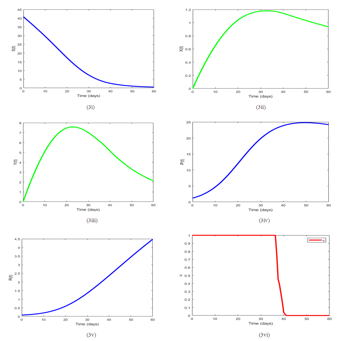 | Figure 3. Simulation results for (1), utilizing the default parameter values outlined in Table 3 and with a control |
In Figure 4., it is observed that, the substrate class, S decreases rapidly within the first few days. This is because more of the pollutants changed their behavior and moved into the X class thereby increasing the content of the X class within the first few days. This occurred upon increasing the transfer rate into the X class, leading to a subsequent reduction in the concentration of pollutants in the tailings dam. Conversely, as the rate of behavior change for the X class increased, lesser control effort was needed to achieve an efficient outcome. This indicates that elevating the transfer rate into the X class may be a productive strategy for curtailing pollutants in the Tailing’s dam.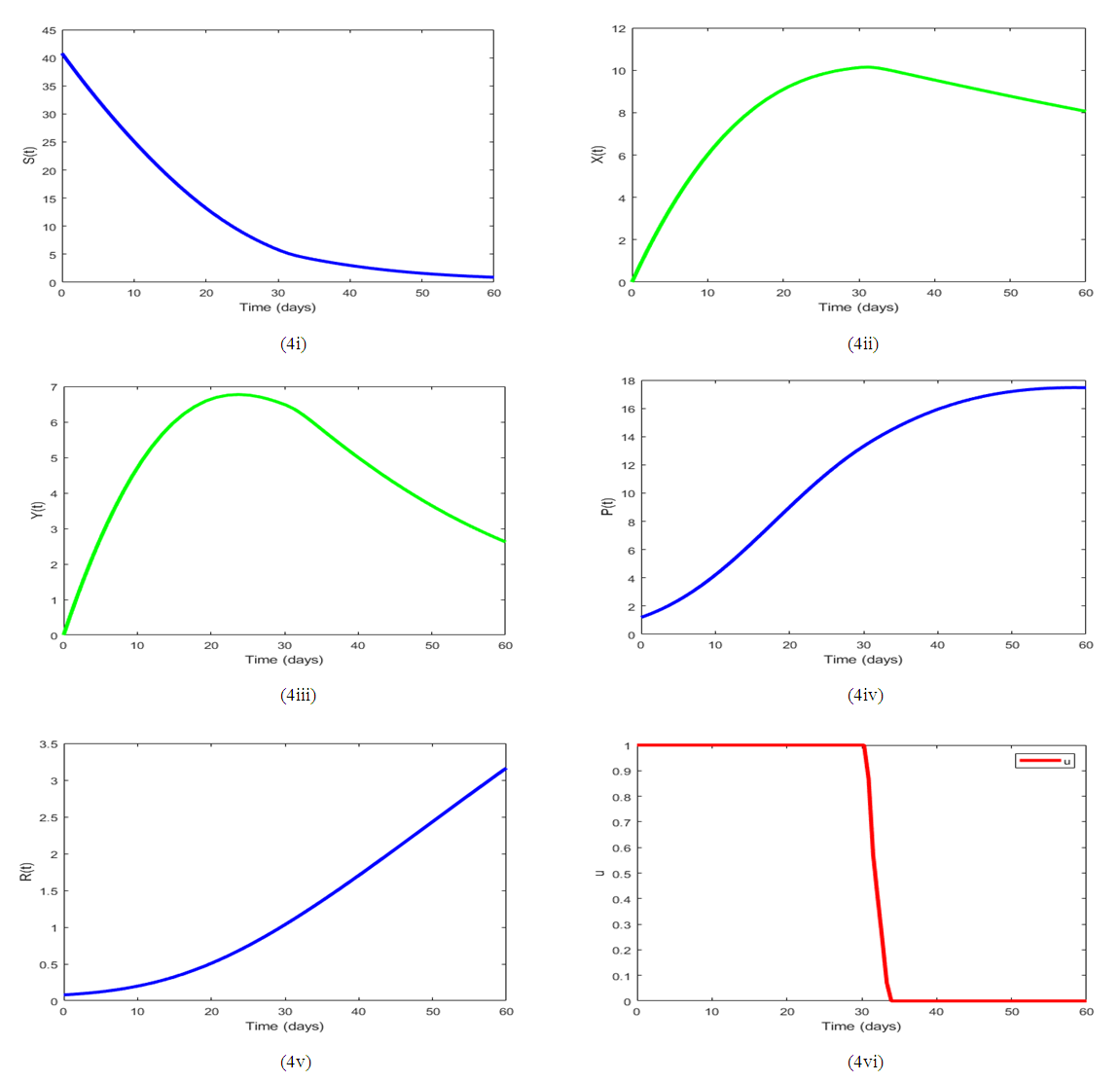 | Figure 4. Simulation results for (1) varying  , utilizing the default parameter values outlined in Table 3 and with a control , utilizing the default parameter values outlined in Table 3 and with a control |
According to Figure 5, upon increasing the input substrate, there was an observable increase in both X and Y classes. This increase in population, however, resulted in a proportional increase in control time from 36 days to about 41 days. Thus, increasing the recruitment rate may potentially lead to a longer control time due to the increased population size. It is, therefore, necessary to exercise prudence when considering the implementation of higher recruitment rates.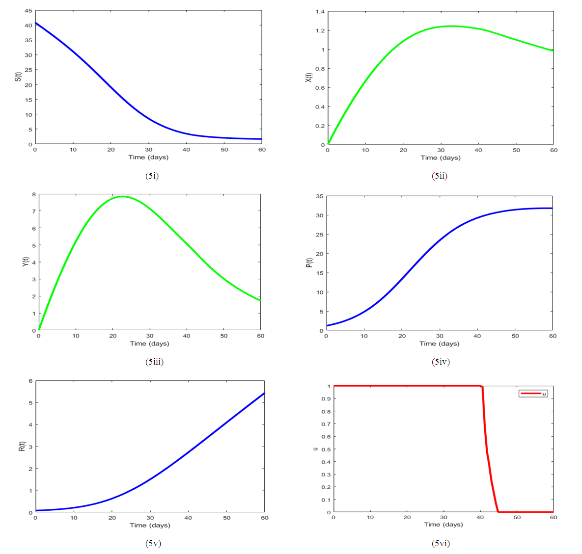 | Figure 5. Simulation results for (1) varying the input substrate utilizing the default parameter values outlined in Table 3, and with a control |
7. Conclusions
A deterministic control model of pollutants in tailings dam has been developed and analyzed for stability. The basic reproduction number was computed to determine the criteria for assessing both local and global stabilities of the model.With the pollution control measure, the basic reproduction number is reduced from 1.60 to 0.8091. This means that the rate of pollution generation is lower than the rate of removal, making the pollutant-free equilibrium (PFE) stable. As a result, pollution levels will gradually decrease over time, leading to a cleaner environment. Optimal control theory has been applied to investigate the optimal strategy for removing or reducing pollutants in the tailings dam using a time-dependent control variable. The simulation results suggest that microbial flocculant is effective for reducing the concentration of pollutants in wastewater treatment processes in the tailings’ dam.
References
| [1] | L. Cosmos, G. Brunetti and B. Liguori, “Assessment of environmental impact of gold production from the urban mining of electronic wastes: a lifecycle assessment approach”, Journal of Cleaner Production, 225, 423-431, doi: 10.1016/j.jclepro.2019.03.087, 2019. |
| [2] | Anon, “Mine Water and Mine Waste Management”, SGU Geological Survey of Sweden, 2021, http://www.sgu.se/en/itp308/knowledge-platform/4-mining-waste/ (Accessed 23/10/2022). |
| [3] | J. Beaudry, “Environmental impact of wastewater discharge from industrial activities”, Journal of Environmental Management, 206, 351-358, doi: 10.1016/j.jenvman.2017.10.012, 2018. |
| [4] | S. R. Shukla, and R. S. Pai, “Adsorption of Cu (II), Ni (II) and Zn (II) on modified jute fibres”, Bioresource Technol 96: 1430–1438, 2005. |
| [5] | K. V. Gupta, M. Gupta and S. Sharma, “Process development for the removal of lead and chromium from aqueous solutions using red mud-an aluminum industry waste”, Water Res 35:1125–1134, 2001. |
| [6] | J. Wang and C. Chan, “Biosorbents for heavy metals removal and their future” Biotechnol Adv 27:195–226, 2009. |
| [7] | M. A. Acheampong, R. J. W. Meulepas, and P. N. L. Lens, “Removal of heavy metals and cyanide from gold mine wastewater”: Review, J Chem Technol Biotechnol, 85: 590–613, doi; DOI 10.1002/jctb.2358, 2010. |
| [8] | P. Anurag, B. Debarbrata, S. Anupam and R. Lalitagauri, “Potential of Agarose for biosorption of Cu (II) in aqueous system”, AmJ Biochem Biotechnol 3:55–59, 2007. |
| [9] | A. Kapoor and T. Viraraghavan, “Fungal biosorption an alternative treatment option for heavy metal cleaning wastewater”, a review. Bioresource Technol 53:195–206, 1995. |
| [10] | K. Song, W. Ma, and S. Guo, “A class of dynamic models describing microbial flocculant with nutrient competition and metabolic products in wastewater treatment”, Adv Differ Equ 2018, 33 https://doi.org/10.1186/s13662-018-1473-6. |
| [11] | A. S. A. Hamzah, A. Banitalebi, and A. H. M Murid, et al., “A Mathematical Model for Wastewater Treatment Process of an oxidation pond”, Proceedings of 3rd International Science Postgraduate Conference 2015 (ISPC2015), 2015. |
| [12] | Z. Tongqian, G. Ning, W. Tengfei, et al., “Global dynamics of a model for treating microorganisms in sewage by periodically adding microbial flocculants”, Mathematical Biosciences and Engineering, MBE, 17(1): 179–201, DOI: 10.3934/mbe.2020010, 2019. |
| [13] | M. Benavente, “Adsorption of Metallic Ions onto Chitosan: Equilibrium and Kinetic Studies”, KTH, Chemical Science and Engineering, TRITA CHE Report 2008:44, 2008. |
| [14] | W. H. Fleming and R. W. Rishel, “Deterministic and Stochastic Optimal Control”, Springer Science and Business Media, Vol. 1, 2012. |
| [15] | C. Castillo-Chavez, Z. Feng and W. Huang, "On the Computation of R0 and its Role on Global Stability. In: Mathematical Approaches for Emerging and Reemerging Infectious Diseases: An Introduction", Springer, New York, pp. 229–250, 2002. |

 Abstract
 Reference
 Full-Text PDF
 Full-text HTML