Herawati N., Saidi S., Setiawan E., Nisa K., Ropiudin
Department of Mathematics, University of Lampung, Bandar Lampung, Indonesia
Correspondence to: Herawati N., Department of Mathematics, University of Lampung, Bandar Lampung, Indonesia.
| Email: |  |
Copyright © 2022 The Author(s). Published by Scientific & Academic Publishing.
This work is licensed under the Creative Commons Attribution International License (CC BY).
http://creativecommons.org/licenses/by/4.0/

Abstract
The rapid development of time series data forecasting methods has resulted in many choices of methods that can be used to forecast according to the type of data. However, what needs to be considered in the selection of forecasting methods is whether the method used provides precise forecasting results or not. The high-order Chen fuzzy time series is a development of the fuzzy time series method with the determination of Fuzzy Logic Relations (FLR) which involves two or more historical data. The back propagation algorithm is one of the algorithms found in the artificial neural network method where this algorithm has a tendency to store experiential knowledge and make it ready for use. This study aims to compare the method of high-order Chen fuzzy time series and feedforward backpropagation neural network in forecasting the composite stock price index based on MSE and MAPE values. The results showed that feedforward backpropagation neural network predicts the composite stock price index better than high-order Chen fuzzy time series method with lower MSE and MAPE values.
Keywords:
High-order Chen fuzzy time series, Feedforward backpropagation neural network, MSE, MAPE
Cite this paper: Herawati N., Saidi S., Setiawan E., Nisa K., Ropiudin, Performance of High-Order Chen Fuzzy Time Series Forecasting Method and Feedforward Backpropagation Neural Network Method in Forecasting Composite Stock Price Index, American Journal of Computational and Applied Mathematics , Vol. 12 No. 1, 2022, pp. 1-7. doi: 10.5923/j.ajcam.20221201.01.
1. Introduction
Forecasting is a method for estimating a value in the future by paying attention to past data. The rapid development of time series data forecasting methods makes researchers have many choices of methods in forecasting data according to their needs. Fuzzy time series is a forecasting method that is often used to predict time series data. This method is based on fuzzy logic [1,2]. High- order Chen fuzzy time series is the development of the fuzzy time series method with the determination of Fuzzy Logic Relations (FLR) which involves two or more historical data [3,4]. Artificial Neural Network (ANN) is an information processing system that has a characteristic appearance that is in accordance with biological neural networks [5]. Meanwhile, backpropagation algorithm is one of the algorithms found in the artificial neural network (ANN) method where this algorithm has a tendency to store experiential knowledge and make it ready to use [6]. The use of high-order fuzzy time series based on neural networks has been done by [7,8,9,10]. In this study, the researchers are interested in comparing high-order Chen Fuzzy Time Series method with the feedforward backpropagation neural network method in forecasting the composite stock price index.
2. Materials and Methods
2.1. Fuzzy Time Series
The fuzzy time series data forecasting method is based on fuzzy logic as a basis. Future data projection with fuzzy time series is done by capturing patterns from past data. The process also does not require a learning system from a complicated system, as in genetic algorithms and neural networks so that it is easy to use and develop [1,2]. In fuzzy time series, several terms are used such as Fuzzy Logic Relations (FLR) and Fuzzy Logic Relations Group (FLRG). FLR is a fuzzy logic that has a relationship between the membership series that have been assigned to the data before and after it. FLRG is a grouping of FLRs based on the value of the previous period. To start forecasting using Chen's time series method, we first have to define a universal set (U) with: | (2.1) |
where  and
and  are are the smallest and the largest data from historical data, respectively.
  and
and  are constant values determined by the researcher. Next, select the classes using the Sturges formula Number of classes = 1 + 3,32
 with Interval length =
  This interval is used to form a number of linguistic values to represent the fuzzy set in the interval formed from the universal set
  where
where  is the universal set and
  is the number of classes with
  The average value of the universal set (U) is:
 | (2.2) |
After that, the fuzzy set must be determined [11]. The fuzzy sets consist of objects in a group class with a continuum of membership degrees. Let  be the universal set, with
  where
where  is the possible value of
  , then variable
  with respect to
  can be formulated as:
 | (2.3) |
 is a membership function of the fuzzy set
  such that
  If
If  is membership of
  then
then  is the degree of membership of
  to
to  Then fuzzification is carried out on historical data to identify the data into fuzzy sets. If the historical data collected is included in the
  interval, then the data will be fuzzified to
  FLR
FLR  is determined based on the
  value that has been determined in the previous step, where
  is data in the previous period and
  is data for next period. For example, if the FLR is in the form of
 then the best FLRG formed is
  After that, defuzzification is performed find the final forecast value using:
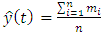 | (2.4) |
where  is defuzzification and
  is the average of
  Finally, perform data forecasting with the following rules: f
  if FLR of
  does not exist
  , then
  . If there is only one FLR
  , then
  and if
  then
then 
2.2. High-order Chen Fuzzy Time Series
To apply high-order Chen fuzzy time series, the calculation steps are identical to Chen's fuzzy time series. However, FLR for high-order is determined by involving two or more historical data [3]. For example, for the second-order it is necessary to involve two historical data, namely  so that FLRG is formed into groups based on the two data. For example if
  and
and  then the FLR formed is
  which is a second-order of FLR.
2.3. Feedforward Backpropagation Neural Network
Artificial Neural Network (ANN) is a network designed to resemble the human brain that aims to carry out a specific task. This network is usually implemented using electronic components or simulated in computer applications. Neural networks are one of the methods used for pattern recognition, signal processing and forecasting, as are other methods found in neural networks. The model of the neural network consists of 3 layers, namely the input layer, the hidden layer and the output layer [6,7].Backpropagation feedforward is a neural network model that can be used in forecasting. Backpropagation was formulated by [12] and popularized by [13] for use in neural networks.The feedforward backpropagation algorithm is referred to as backpropagation because when the network is given an input pattern as a training pattern, the pattern goes to the units in the hidden layer to be forwarded to the output layer units [14]. Furthermore, the output layer units provide a response which is known as network output, when the network output is not the same as the expected output then the output will spread backward in the hidden layer forwarded to the units in the input layer.To construct an artificial neural network using the feedforward backpropagation algorithm is to first determine the input based on the significant lags in Partial Autocorrelation Function Plot (PACF). Next, divide data into training and testing data. Percentage of Composition of training and testing data is open, can be 80-20 or 70-30 or 50-50. Before doing so, the data needs to be normalized. Normalization of data can be done with the following transformation formula: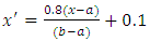 | (2.5) |
where  is normalized data and
  is data to be normalized, respectively.
  and
and  are the minimum and maximum values of the data. Furthermore, the activation function and training algorithm have to be determined. The selection of the activation function must meet the conditions of being continuous, differentiable and not descending. The activation function is used in the first (hidden) and second (output) layers. While the training algorithm is used for the training stage. Next, the model is formed through the training stage by changing the number of hidden layers. Determination of the number of hidden layers is done by looking at the smallest error value. MAPE is used to measure the level of model reliability, while MSE is used to measure the accuracy of learning outcomes from the model. The best model obtained based on the smallest MAPE and MSE values at the training stage is used to form a model at the testing stage.After getting the best model from the training stage, the next step is to carry out the testing stage to determine the accuracy or error rate of the model obtained at the training stage and carry out the forecasting process. In the forecasting process, all the data used to get the forecasting process for the next period is still in the form of normalized data. Forecasting results in the form of normalized data must be denormalized in order to obtain the original value data from the forecasting results. Forecasting results can be denormalized using formula:
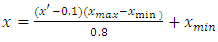 | (2.6) |
with  is normalize values in the dataset,
  and
and  are the minimum and maximum values, respectively.
2.4. Forecasting Accuracy Measure
In order to produce optimal forecasting with a small error rate, Mean Square Error (MSE) and Mean Absolute Percentage Error (MAPE) are calculated and compared from both methods with the following formula: 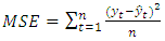 | (2.7) |
where  and
and  are the actual values in the ke-t period and the forecasted values in the ke-t periods, respectively.
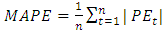 | (2.8) |
with 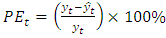 .
.
3. Results and Discussion
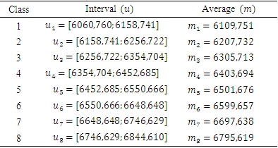
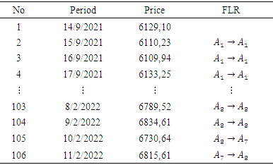
The composite stock price index data from the period September 2021 to February 2022 obtained from https://finance.yahoo.com/quote/%5EJKSE/history/ was analyzed using high-order Chen time series fuzzy method and feedforward backpropagation neural network method using R-Studio software and Matlab R2013a.The first step was to predict the data using a high-order fuzzy Chen time series method. To forecast using this method, we must first determine the universal set (U) according to the definition in equation (2.1) and we obtained U = [6060,76;6844,61]. Then the universal set U is divided into classes to look for the average value in each class. The resulting classes of the universe set is:Table 1. The Universal Set (U)
 |
| |
|
Based on the rules of determining the degree of membership of the fuzzy set formed are as follows: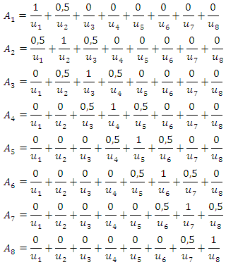 Next, fuzzification was carried out on the data and the results are obtained in Table 2.
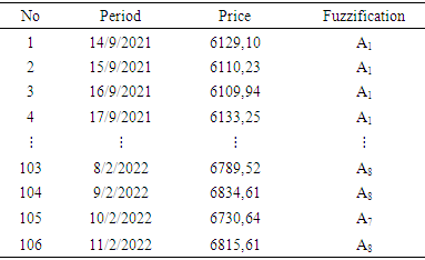
Table 2. Fuzzification of Composite Stock Price Index Data
 |
| |
|
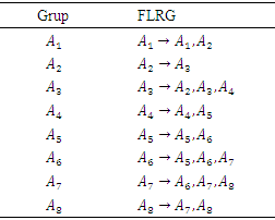
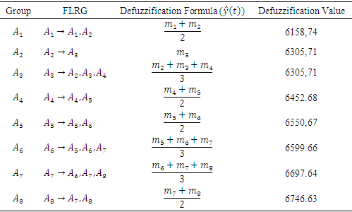
Then the next step was to define the Fuzzy Logic Relations (FLR) and Fuzzy Logic Relations Group (FLRG) and defuzzification. The results are shown in Table 3-6.Table 3. FLR Composite Stock Price Index Data
 |
| |
|
Table 4. FLRG Composite Stock Price Index Data
 |
| |
|
Table 5. FLRG Defuzzification
 |
| |
|
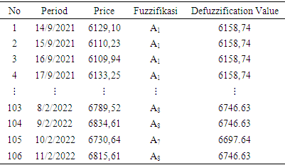
Table 6. Defuzzification of Composite Stock Price Index Data
 |
| |
|
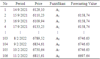
Next, forecasting was carried out in the first-order and the results are as presented in Table 7.Table 7. First-order forecasting on composite stock price index data
 |
| |
|
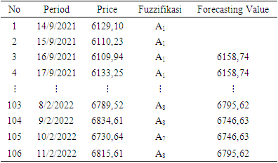
The next step was to forecast the second and third-order using the same universe set. In this high-order forecasting method, it starts with determining the Fuzzy Logic Relations (FLR) and the Fuzzy Logic Relations Group (FLRG). The results of forecasting the composite stock price index data using a high-order Chen fuzzy time series can be seen in Table 8-9.Table 8. Second-order forecasting on composite stock price index data
 |
| |
|
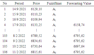
Table 9. Third- order forecasting on composite stock price index data
 |
| |
|
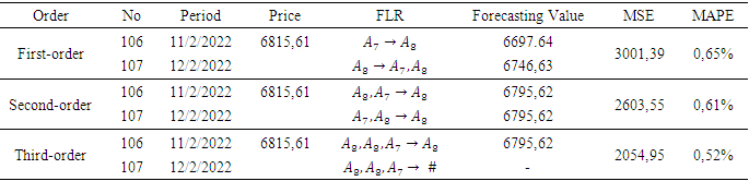
The predicting data was obtained by looking at the FLR in the previous period and match it with FLRG. For example, in the period of February 11, 2022, we had FLR  so that in the period of February 12, 2022, the forecasting value used is in Group
  with the relation
  In the second-order, the determination of the forecasting value for the future period is done by looking at the FLR in the previous period. Meanwhile, the determination of the forecast value for the next period in the third-order is carried out in the same way but by using two data from the previous period. The following are the results of data forecasting using a high-order Chen fuzzy time series.Based on Table 10, it can be seen that the third order produces forecasting values with the smallest MSE and MAPE. However, it cannot predict the data for the next period which is denoted by (#) because the resulting relation in the next period does not exist in the predefined group or groups in the third-order FLRG. Therefore, forecasting stops in the second-order.
Table 10. Composite stock price index forecast results on high-order
 |
| |
|
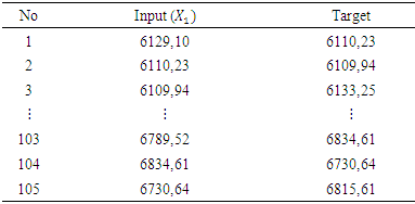
Furthermore, the data were analyzed using the feedforward backpropagation neural network method. The first step is to determine the network input by looking at the significant lag in PACF plot. Figure 1 shows that the significant PACF plot is at lag 1 and the network input is at  Based on this, the network input was defined as seen in Table 11.
Table 11. Network Input
 |
| |
|
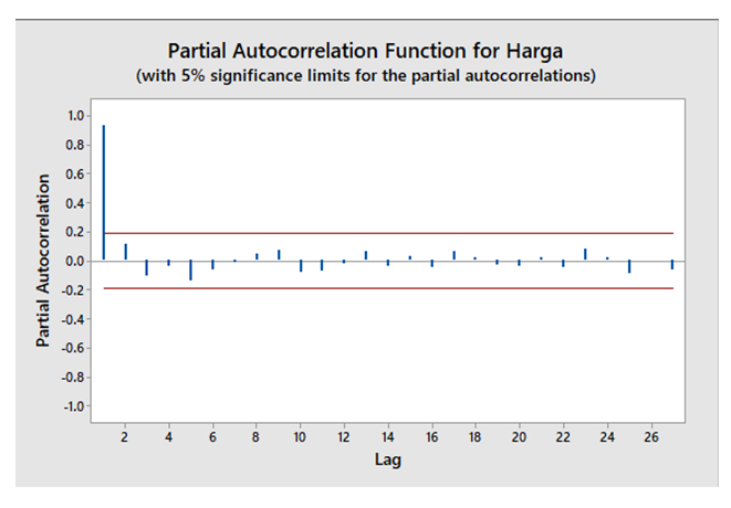 | Figure 1. Plot of PACF Composite Stock Price Index Data |
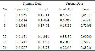
After that, the data were analyzed using a feedforward backpropagation neural network method. The first thing to do was divide the data into training data and test data with a percentage of 70% training data and 30% test data. Then normalization was carried out on the two data as shown in Table 12.Table 12. Normalization Results
 |
| |
|
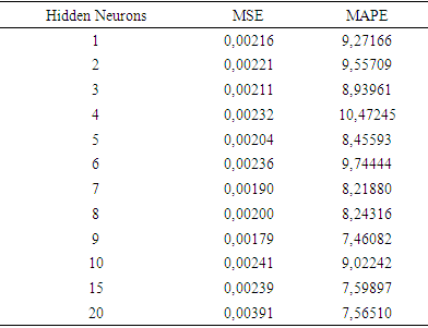
After the normalization process is carried out, the next step was to define the activation function and training algorithm. The activation function used in the hidden layer was binary sigmoid (tansig) and the output layer used an identity or linear (purelin) activation function. Meanwhile, the training algorithm used trainlm. Next was the formation and selection of models based on the MSE and MAPE values at the hidden neurons training stage. The following are some of the models built as presented in Table 13.Table 13. MSE and MAPE Values on Hidden Neurons Training Stage
 |
| |
|
Table 13 shows that the smallest MSE and MAPE values in 9 hidden neurons. Therefore, feedforward backpropagation neural network model was formed using 1 input layer, 9 hidden layers and 1 output layer.After getting the best model at the training stage, the next step was to calculate the weight of maximum epoch value (iteration) of the model at the training data using the parameters obtained. The resulting weight was 1000 and shows 25 with a performance goal of 0.001, a learning rate of 0.01 and a momentum constant of 0.9. Table 14 gives the results of the weight values obtained using these parameters.Table 14. The Weight values
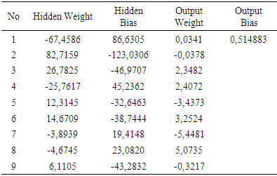 |
| |
|
The next stage of testing was carried out to determine the accuracy or error rate of the best model obtained at the training stage by looking at the forecasting data at the resulting test stage. Forecasting calculations at the testing stage are carried out using 31 data with weights that have been obtained from the training stage as seen in Figure 2. 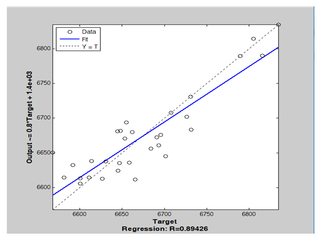 | Figure 2. Correlation in testing stage |
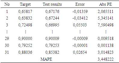
Figure 2 shows that the correlation is 0.89426. It means that the target data and the test results data at the testing stage have a good correlation. It also indicates that the accuracy between the target data and the test result data is high. While Figure 3 shows that there is no significant difference between the target data and the test result data. Table 15 presents a comparison between the target data and the test results at the testing stage. In addition, we can see MAPE's value is 3.448222%. This shows that the level of accuracy is quite high because it is below 10%. 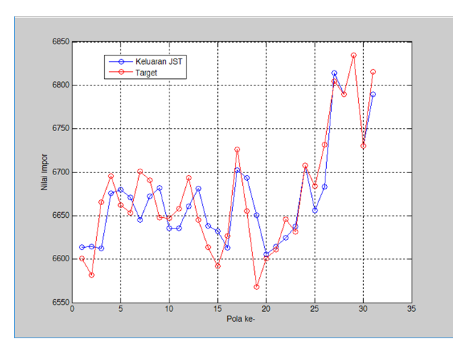 | Figure 3. Comparison of target data with test results at the testing stage |
Table 15. Comparison of Target Data with Test Results at the Testing Stage
 |
| |
|
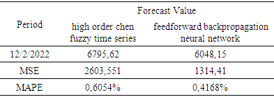
After the training and testing stages are carried out, forecasting is carried out for the period 12 February 2022. Forecasting value for this period is 6048.15. This forecast uses the overall data using the best model and the parameters obtained. Finally, we compared the forecasting accuracy between high-order Chen fuzzy time series and a feed-forward propagation neural network based on MSE and MAPE as presented in Table 16.Table 16. Forecasting value comparison
 |
| |
|
Table 16 shows that feedforward backpropagation method has MAPE = 0.4168% and MSE = 1314.41 and high-order Chen fuzzy time series has MAPE = 0,6054% and MSE = 2603,551, respectively. This shows that feedforward backpropagation neural network method performs better than high-order Chen fuzzy time series with smaller MAPE and MSE. Therefore, what we use to estimate the composite stock price index for the next period is based on feedforward backpropagation, which is 6048.15.
4. Conclusions
Based on the results of the analysis of the two methods used, it can be concluded that the feedforward backpropagation forecasting method has better performance than the high-order fuzzy Chen time series forecasting method. The error values of Mean Square Error (MSE) and Mean Absolute Percentage Error (MAPE) of the feedforward backpropagation method are lower than the high-order Chen fuzzy time series forecasting method. This method produces MSE = 1314.41 and MAPE = 0.4168% with the forecast value in the next period is 6048.15. Meanwhile, in the high-order Chen fuzzy time series forecasting method, MSE = 2603.551 and MAPE = 0.6054% with a forecasting value of 6795.62.
References
| [1] | Song, Q. and Chissom, B. S. 1994. Forecasting Enrollments with Fuzzy Time Series-Part II, Journal of Fuzzy Sets and System, 62(1), 1-. |
| [2] | Chen, S. M. 1996. Forecasting Enrollments Based on Fuzzy Time Series. Journal of Fuzzy Sets and System. 81(3): 311-319. |
| [3] | Chen, S.M. 2002. Forecasting Enrollments Based on High-Order Fuzzy Time Series, Cybernetics and Systems, 33(1), 1-16. |
| [4] | Chen S.M., Chung N.-Y. 2006. Forecasting enrollments using high-order fuzzy time series and genetic algorithms, Int. J. Intell. Syst., 21 (5), 485-501. |
| [5] | Fausett, L. 1994. Fundamentals of Neural Networ, Architecture, Algoritm and Application. London: Printice-Hall Inc. |
| [6] | Alexander, I. and Morton, H. 1994. Neural Networks: A Comprehensive Foundation. New York: Springer Verlag. |
| [7] | Aladag, C.H., M.A. Basaran, M.A., E. Egrioglu, E., U. Yolcu, U., and Uslu, V.R. 2009. Forecasting in high order fuzzy time series by using neural networks to define fuzzy relations. Expert Syst. Appl., 36, 4228-4231. |
| [8] | Chen, M.Y. 2014. A high-order fuzzy time series forecasting model for internet stock trading, Future Generation Computer Systems, 37, 461-467. |
| [9] | Yu T.H.K. and Huarng K.H. 2010. A neural network- based fuzzy time series model to improve forecasting, Expert Syst. Appl., 37, 3366-3372. |
| [10] | Aladag, C.H., Yolcu, U., and Egrioglu, E. 2010. A high order fuzzy time series forecasting model based on adaptive expectation and artificial neural networks, Math. Comput. Simul, 81, 875-882. |
| [11] | Zadeh L.A. 1965. Fuzzy Sets. Information and Control, 8, 338-353. |
| [12] | Werbos, P. “Beyond regression: New tools for prediction and analysis in the behavioral sciences,” Ph.D. dissertation, Committee on Appl. Math., Haivard Univ., Cambridge, MA, Nov. 1974. |
| [13] | Rumelhart, D. E., Hinton, G. E., and Williams, R. J., 1986, Learning internal representations by error propagation, in Parallel Distributed Processing: Explorations in the Microstructure of Cognition, vol. 1, Foundations, (D. E. Rumelhart, J. L. McClelland, and PDP Research Group, Eds.), Cambridge, MA: MIT Press, chap. 8. |
| [14] | Yu, X., Efe, M. and Kaynak, O. 2002. A general backpropagation algorithm for feedforward neural network learning. IEEE Transactions on Neural Networks, 13(1): 251 – 254. |

 Abstract
 Reference
 Full-Text PDF
 Full-text HTML