Jay P. Narain
Retired, Worked at Lockheed Martin Corporation, Sunnyvale, CA, USA
Correspondence to: Jay P. Narain, Retired, Worked at Lockheed Martin Corporation, Sunnyvale, CA, USA.
| Email: |  |
Copyright © 2021 The Author(s). Published by Scientific & Academic Publishing.
This work is licensed under the Creative Commons Attribution International License (CC BY).
http://creativecommons.org/licenses/by/4.0/

Abstract
The neural network solution method is applied to solve coupled non-linear differential equations for a free convection problem on a stationary wall. The results show good comparison with results from other published methods. Next a finite difference equation solver is extended to three and four dimensions. The code is tested for zero Dirichlet boundary condition and mixed non-zero Dirichlet and Neumann boundary conditions cases. The results are compared with neural network solutions with satisfactory outcome. The finite difference equation has also been extended to polar coordinates to solve potential flow problem over a two-dimensional infinite cylinder. The results are excellent.
Keywords:
Differential equations: non-linear ordinary and partial, Neural netwok, Finite difference equations in polar, Three and four diemensions
Cite this paper: Jay P. Narain, Comparison of Neural Network and Finite Difference Solutions, American Journal of Computational and Applied Mathematics , Vol. 11 No. 3, 2021, pp. 65-70. doi: 10.5923/j.ajcam.20211103.03.
1. Introduction
The ordinary and partial differential equations have been solved anaytically and numerically for many years. Various numerical schemes were developed with the advent of computers. From such schemes, the finite difference scheme has been a popular numerical method. The boundary condition based neural network method for non linear Blasius equation was investigated by Kitchin [1]. This work was extended to more complicated Falkar-Skan equations by Narain [2]. The neural network method is capable of solving coupled non-linear differential equations as well as ordinary to partial differential equations. There are numerous applications of neural network method to solve fractional differential equations in literature. Most of the finite-difference solvers are limited to two-dimensional domain. Extension of finite difference method to higher dimension will be desirable for analysis purposes. This will help in improving the neural network prediction capability. The finite difference runtime efficiency is extremely high in comparison to neural network solution. However, neural network solutions maintain high accuracy in any dimension irrespective of grid dimensions.
2. Discussions
Next, we will discuss a new non-shooting method which works well for most linear and nonlinear differential equations [1,2]. We will solve a set of coupled thermal boundary layer equations for free convection thermal boundary layer over a stationary flat plate. Derivation of the governing equations can be found in Deen’s book [3]. In the Boussinesq approximation for an incompressible fluid and a steady-state regime, the equations of momentum, mass and energy conservation for laminar free convection in a plane boundary layer are as follows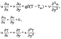 | (1) |
We shall reduce the equations to the dimensionless form. It is convenient to use the quantities entering into the unambiguity conditions (boundary conditions) as the reduction scales. As a linear scale we shall take some characteristic dimension of a body L, for a temperature it is convenient to use, for instance, the relation θ = (T – T∞)/(Tw – T∞), where Tw is the body surface temperature, T∞, is the surrounding temperature, T is the local temperature. The characteristic velocity may be obtained from the comparison of volumetric and viscosity forces u0 = βgΔTL2/ν or from the estimates of the type u0 = L/τ0, where τ0 is the time scale. The dimensionalization yields: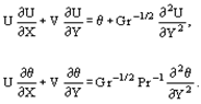 | (2) |
The Grashof number Gr = βgΔTL3/ν2 is the main governing criterion and the most important characteristic of free convection heat transfer. It is the measure of the relation between the buoyancy forces in a non-isothermal flow and the forces of molecular viscosity. It also determines the mode of medium motion along the heat transfer surface. In its physical meaning, it is similar to the Reynolds number for a forced flow.A specific feature of laminar free convection on a vertical plate at a constant wall temperature is the fact that it allows a self-similar solution if a new variable is introduced into above equations in the form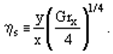 The boundary conditions are
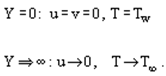 Having represented the stream function and the dimensionless temperature as
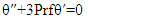
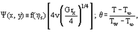 we obtain Eqs. (1) in the form
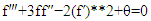 | (3) |
 | (4) |
with the boundary conditions: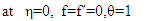 | (5) |
 | (6) |
where f’, f’’, and f’’’ are first, second and third derivatives, * and ** denote multiplication and exponential mathematical operation.This problem was solved originally by Ostrach [4]. Sparrow and Gregg [5] also solved this problem and found their results in agreement with experimental data. The present numerical scheme consists of two neural networks, one for stream function f and another for modified temperature function θ.  The results are carried out for Pr=0.1, 1.0, and 10. It took about 620 s on an Intel i7-6700T, 2.8 Ghz, 8 GB ram home personal computer.We will compare the results of our neural network with a well-known solver [8,9] “fsolve” which is used to find root of an equation. Only a few iterations are required with this method, to iteratively solve the coupled equations and get a good solution. This is a non-shooting, non-machine learning method scheme which uses finite difference form of equations and takes lot less run time. It took only 47.7 s to solve. The results are compared for both the schemes and are presented in the following figures.
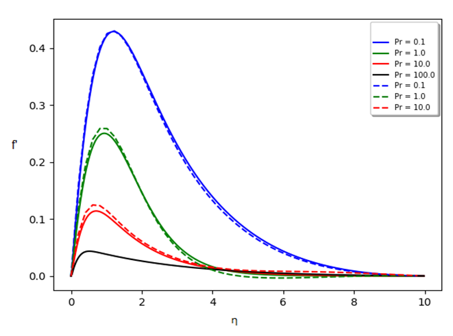 | Figure (1). Comparison of velocity(f’) profile from neural network (-- lines) and “fsolve” (solid lines) solvers |
The case for Pr = 100 did not run with the neural network. 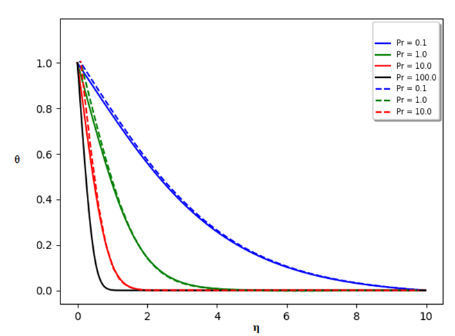 | Figure (2). Comparison of modified temperature profile with the two schemes |
In conclusion, the finite difference solvers are computationally more efficient and stable. On the other hand, the neural network method does not require knowledge of any numerical methods, such as finite difference, and are easy to set up. Overall, the neural network method is quite slow and needs considerable improvement in computational efficiency in future. The code has been hosted in narain42/Machine-learning-methods-in-Fluid-Dynamics on GitHub.Recently the solution of Poisson’s equation was presented in three and four dimensions using neural network scheme [10]. The computational time was staggering and of some concern for their practicality. Presently we will develop iterative finite difference solver up to four dimensions using known solution methods such as Jacobi, Gauss-Seidel, Gradient descent and Conjugate gradient. A base two-dimensional code [11] was extended to higher dimensions. The basic two-dimensional Jacobi Poisson’s equation iterator was for similar grid in two dimensions(dx=dy). Here the grid spacing in two dimensions are kept distinct.;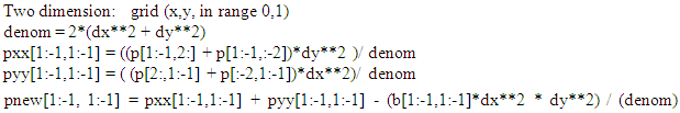 | (7) |
where dx and dy are the grid spacing increment, p is the solution function, pxx and pyy are the second derivative of p with respect to x and y, and b is the source function for a typical Poisson’s equation. pnew is the iterative update in Python subject to the following boundary conditions: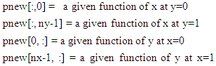 | (8) |
For a contrived test case with equation f(x,y), the source function b(x,y) is Laplacian (pxx+pyy) of the function f(x,y). The boundary conditions can be easily derived by setting x,y values in the f(x,y). In reality, the exact function f(x,y) will not be known in advance, but the boundary conditions and the source function will be known for a given scenario.The extension to three dimension and four dimensions is as follows:Three dimension: grid (x,y,z in range 0,1)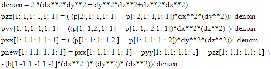 | (9) |
#Boundary Conditions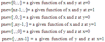 | (10) |
where dx, dy, and dz are the grid spacing increment, p is the solution function, pxx ,pyy and pzz are the second derivative of p with respect to x, y, and z, and b is the source function in a typical Poisson’s equation. pnew is the iterative update for p. The equations are written in Python: The extension to four dimensions is routinely intuitive and will be provided in GitHub repository. Presently three-point central differencing is used which is second order accurate. Higher order differencing 14 to 27 order have been published for three-dimension case to solve Poisson’s equations using matrix inversion. [12]The Gauss-Seidel scheme follows same equations, where some of the explicit terms are replaced with implicit terms. With the Pythonic vectorization., the results and run times are similar to Jacobi iterative scheme.The Gradient descent and Conjugate gradient are very powerful and run time efficient schemes. They are limited to any dimensional case with zero Dirichlet boundary conditions. It only requires the Poisson’s operator A(v), and source function b. The A(v) is extended as follows: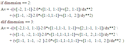 | (11) |
The solution procedure is very short and is defined in the code.The present computational methods are compared with the neural network for a zero Dirichlet case and a case with non-zero boundary conditions.Case 1: Zero Dirichlet Boundary conditions: The analytical function will be sin(pi*x)*sin(pi*y)*sin(pi*z)*sin(pi*t). This function can be used for any dimension by deleting extra dimension in the function, like for two dimension use sin(pi*x)*sin(pi*y). The grid size is (31x31x31x31) with order reduction for lower dimension analysis. Accuracy is determined as follows consistent with that used in neural network solutions [10].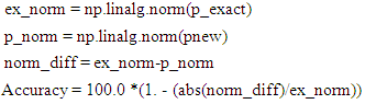 | (12) |
where p_exact is the contrived analytical function, pnew is the derived solution, linalg.norm is a numpy function which returns the norm of a vector or matrix.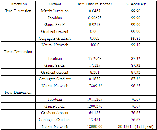 The accuracy seems to decrease with higher dimensionality. Obviously higher order difference schemes will improve the results. The neural network solutions show much better capability and are insensitive to grid size used. Above table shows that in four-dimensional case, a coarse (4(11)) grid gives better solution than (4(31)) grid used in finite difference solution.Case 2:
 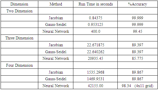 Non-zero Mixed Dirichlet and Neumann Boundary conditions: The analytical function will be exp(-x)*(x + y **3 + z**3 + t**3) This function can be used for any dimension by deleting extra dimension in the function, like for two dimension, use exp(-x)*(x + y **3) The grid size is (31x31x31x31) with order reduction for lower dimension analysis. Accuracy is determined by using equation (12). Only Jacobian and Gauss Seidel results will be compared with neural network since gradient descent and conjugate gradient capability are limited to zero Dirichlet boundary conditions. Matrix inversion method was not attempted for higher dimensions.The accuracy seems to decrease with higher dimensionality. Obviously higher order difference schemes will improve these results. The neural network solutions show much better capability and are insensitive to grid size used. Above table shows that in four-dimensional case, a coarse (4(11)) grid gives better solution than (4(31)) grid used in finite difference solution.Case 3:Most of the neural network analysis is done in cartesian coordinate. Even the regression theory uses cartesian concept. A solution of potential fluid flow over a cylinder has a Laplacian in polar coordinate with source term equal to zero. An attempt to analyze this problem with neural network was partially successful [10]. Even the finite difference formulation runs into problem because of the nature of the equation below:
 | (13) |
where polar coordinates are radius r and angle θ. The coding of second and first derivative is straight forward in finite difference scheme. The coefficients (1/r) and (1/r^2) create problem in Pythonic vector notation. Since r is always positive, we can assume these as coefficients and use them as variable scalar quantities. With the coding notation of x as r and y as theta, the following Python code gives the finite difference operator in polar coordinate: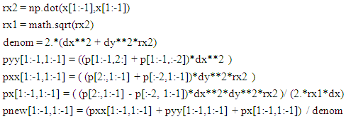 | (14) |
The equation (13) has a simple closed form solution on a cylinder of radius one and is given by [13];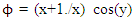 | (15) |
In equation (14) ϕ is represented by p and pnew in iteration process. With the known exact solution, the boundary conditions on a r or x (1,60) and θ or y (-pi,pi) grid are given by,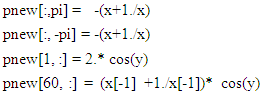 | (16) |
where x[-1] refers to outer radial boundary, and the parameters in pnew have been altered for theoretical depiction.The iterative solution took 0.9531 s and had the accuracy of 96.8175%. The neural network [10] run time was 400 s and accuracy of 91.6%. Presently extending the outer limit of r to higher values and increasing number of grid points in radial direction slightly improves the accuracy. The following figure shows the results for ϕ.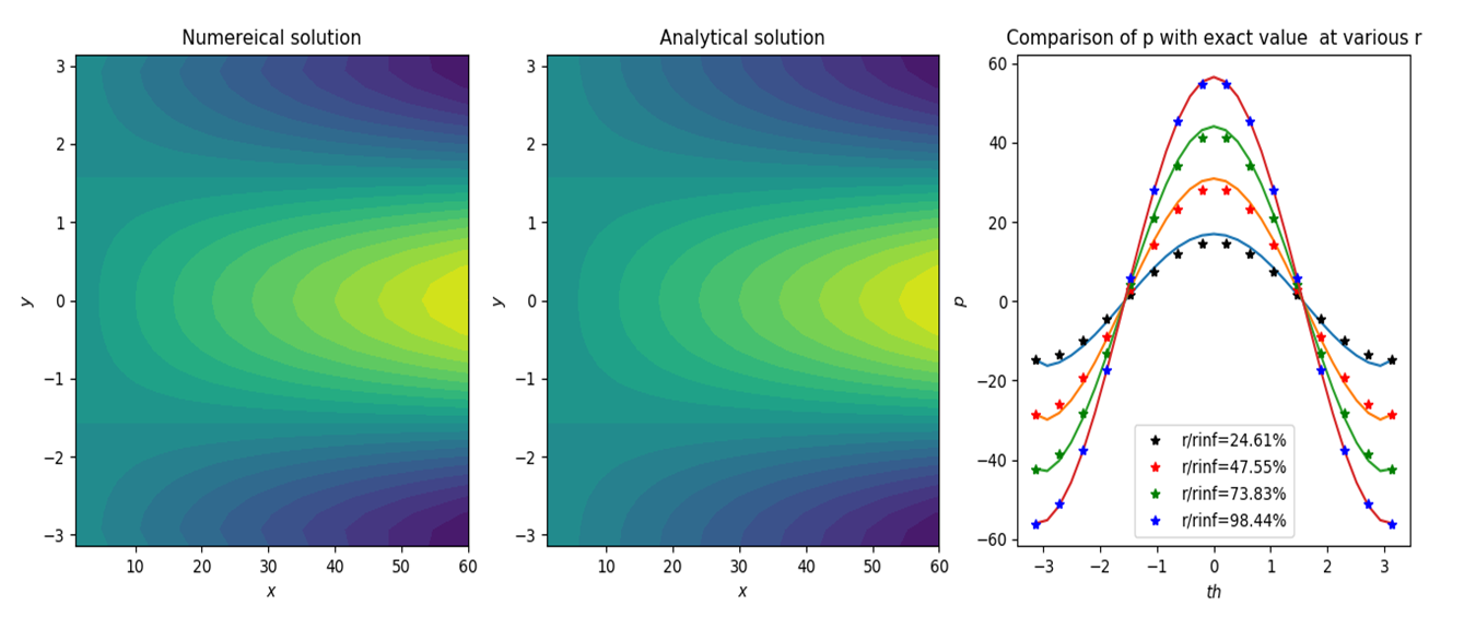 | Figure (3). Solution of potential flow over a cylinder |
The code for all the iterative analysis has been posted in narain42/Poission-s-Equation-Solver-Using-ML as new iterative_methods_rev.py on Github.
3. Conclusions
The neural network seems to have excellent predictive capability in coupled non-linear differential equations. The free convection from a vertical flat plate results from this method and a method using “fsolve” shows excellent correlation. The extension of finite difference solution to higher dimension shows promising capability. The comparison of two test cases showed that the accuracy in finite difference decreases with higher dimensions. The finite difference runtime efficiency is extremely high in comparison to neural network solution. However, neural network solutions maintain high accuracy in any dimension irrespective of grid dimensions. The potential flow over a cylinder in polar finite difference scheme showed better result compared to neural network solution [10].
References
| [1] | John Kitchin, “/kitchingroup.cheme.cmu.edu/blog/2017/11/27/Solving-BVPs-with-a-neural-network-and-autograd/”, 11/27/2017. |
| [2] | J.P. Narain, “Exploring Blasius and Falkner-Skan Equations with Python”, American Journal of Fluid Mechanics, Feb 6, 2021. |
| [3] | William M. Deen, “Analysis of Transport Phenomena”, Oxford University Press, 1998". |
| [4] | Ostrach,“An analysis of laminar free-convection flow and heat transfer about a flat plate parallel to the direction of the generating body force”, NACA Tech. Rept. No 1111, 1953. |
| [5] | Sparrow and Gregg 5 “J. Heat Transfer”, 1956, v. 78, p. 435. |
| [6] | Ryan Adams, “autograd”, HIPS/autograd on github.com”, March 5, 2015. |
| [7] | Diederik P. Kingma, Jimmy B,”Adam: A Method for Stochastic Optimization”, arxiv, 2015. |
| [8] | Powell, M. J. D., "A Fortran Subroutine for Solving Systems of Nonlinear Algebraic Equations," Numerical Methods for Nonlinear Algebraic Equations, P. Rabinowitz, ed., Ch. 7, 1970. |
| [9] | Moré, J. J., B. S. Garbow, K. E. Hillstrom,” User Guide for MINPACK 1”, Argonne National Laboratory, Rept. ANL-80-74, 1980. |
| [10] | J.P. Narain,” Solution of Poisson’s Equation In Higher Dimensions Using Simple Artificial Neural Network”, American Journal of Computational and Applied Mathematics, 2021, 11(3): 51-59. |
| [11] | “http://33h.co/9nak1” |
| [12] | A. Shiferaw, and R.C. Mittal,”An efficient direct metod to solve the three dimensional Poisson’s equation”, American Journal of Computational mathematics, December 2011. |
| [13] | A.M. Keuthe and C.Y. Chow., “Foundations of Aerodyanics,” Fifth Edition, 1998. |

 Abstract
 Reference
 Full-Text PDF
 Full-text HTML