Jay P. Narain
Retired, Worked at Lockheed Martin Corporation, Sunnyvale, CA
Correspondence to: Jay P. Narain, Retired, Worked at Lockheed Martin Corporation, Sunnyvale, CA.
| Email: |  |
Copyright © 2021 The Author(s). Published by Scientific & Academic Publishing.
This work is licensed under the Creative Commons Attribution International License (CC BY).
http://creativecommons.org/licenses/by/4.0/

Abstract
The use of artificial neural network to solve ordinary and elliptic partial differential equations has been of considerable interest lately [1,2,3,4,5]. The error loss optimization techniques [6,7] usually reach an undesirable minimum at some point. Further convergence is usually sought with other minimization [8]. schemes. The use of BFGS scheme has been presently investigated. The simple artificial neural network [4,5] has been applied to solve problems in higher 3 to 4 dimensions with relative ease. The results show a promising trend. The potential flow over an infinite 2D cylinder in polar coordinates has also been investigated. One would expect exact comparison with analytical solution for such a simple problem. However, due to poor convergence, the use of cartesian based neural network for polar coordinate correlation becomes an issue.
Keywords:
Ellpitic partial differential equations, Solution in higher dimesions, Neural network, Machine learning methods
Cite this paper: Jay P. Narain, Solution of Poisson’s Equation in Higher Dimensions Using Simple Artificial Neural Networks, American Journal of Computational and Applied Mathematics , Vol. 11 No. 3, 2021, pp. 51-59. doi: 10.5923/j.ajcam.20211103.01.
1. Introduction
The neural network schemes require derivative of neural network. The autograd researchers [4] and Angel [6] have provided nice automatic differentiation schemes. The boundary condition embedded artificial neural network scheme [1] (ANN) works nicely on ordinary and partial differential elliptic equations up to second order. Our explicit boundary condition with simpler neural network scheme [4,5] has shown similar promise. The extension of simpler neural network scheme [4,5] to three- and four-dimensional equations is relatively an easy task, whereas more theoretical work will be needed for the ANN [1] scheme. There are relatively only a few research works in solving Poisson’s equation in higher dimensions. The finite difference formulation for a three-dimensional case [9] shows the complicated nature of formulation The convergence of numerical solutions on minimization schemes and activation function is also discussed. Since most of the regression in neural network is based on cartesian grid data correlation, its impact is shown in the solution of potential flow solution on an infinite cylinder in polar coordinates. A need to develop general grid free correlation is highly desired (not attempted here).
2. Discussions
Case A: First we will be studying impact of minimization schemes in boundary condition-based solution of Poisson’s equation [4,5]. The automatic differentiation scheme of neural network will be used [4,6], The basic model of the study for reference is as follows:Exact Contrived solution: 𝛟 = x**2+y**3With the assumed exact solution, the source term and the boundary conditions specifications become simple task. Taking the second derivative with spatial coordinates and adding them makes the source term f shown below. The Dirichlet boundary condition is merely a substitution of proper control point value in exact solution. For example, bc (at y=0) shown below, is obtained by just replacing y to zero in exact solution. For Neumann boundary condition proper derivative and boundary condition has to be prescribed [3]. In practical situations, the exact solution is not known in advance. However, with the known source function and boundary conditions, the Poisson’s equation can be solved. For comparison purposes, a simple finite difference scheme will give adequate solution in place of exact solution.Source term (right hand side of Poisson’s eq.): f = 2. + 6*yLaplace operator (left hand side eq.): d2 𝛟(x,y)/dx2 + d2 𝛟(x,y)/dy2 Boundary conditions: Dirichlet boundary conditions for (1,1) square domain is:bc(at y=0) = x**2bc(at y=1) = (x**2+1.) bc(at x=0) = y3bc(at x=1) = (1.+y3) The basic solution converges reasonably fast. The Adam [7] optimization using error loss reduction, gives reasonably converged solution in 50 iterations. Further convergence can be obtained by using BFGS and other minimization schemes [8]. In the first run, the Adam optimization alone reduced the loss error to 9.021e-03 in about 400 sec of computer run time. Further convergence was sought with BFGS method. It took additional 2 hrs. and 36 mins to reduce the error to 2.8745e-05. The heatmap of difference in exact and numerical solution and predictions at few cross sections are shown below.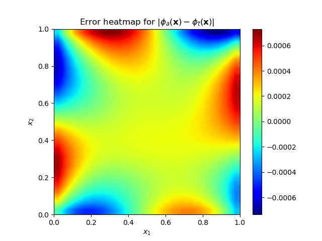 | Figure 1(a). Heat map of prediction and exact solution error |
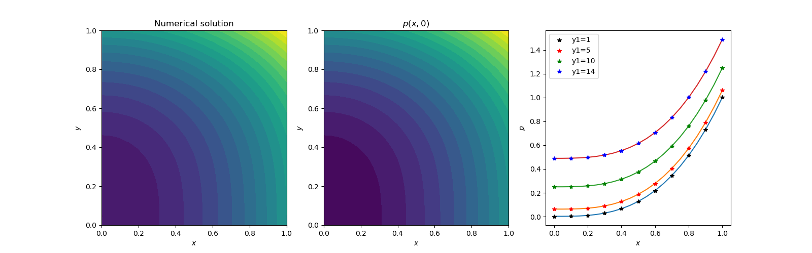 | Figure 1(b). Contour plots of exact and numerical solutions and cross section data comparison |
The excessive use of run time over two and half hour was alarming. Although this approach is used frequently in analysis [2], the run time will be very short if the error loss has converged to the order of 1.e-05 or 1.e-06. Another alternative will be to use Adam and BFGS method simultaneously and limit the number of iterations to 3 to 5 iterations in the inner loop. For the outer loop, any number of Epochs (Iterations) can be prescribed. We will use 30 Epochs, with 5Adam iteration and 3 BFGS iterations. The error loss converged to 3.196e-05 in 36 sec of run time. Although the heat map errors are higher, the section data comparison is acceptable for most engineering purposes.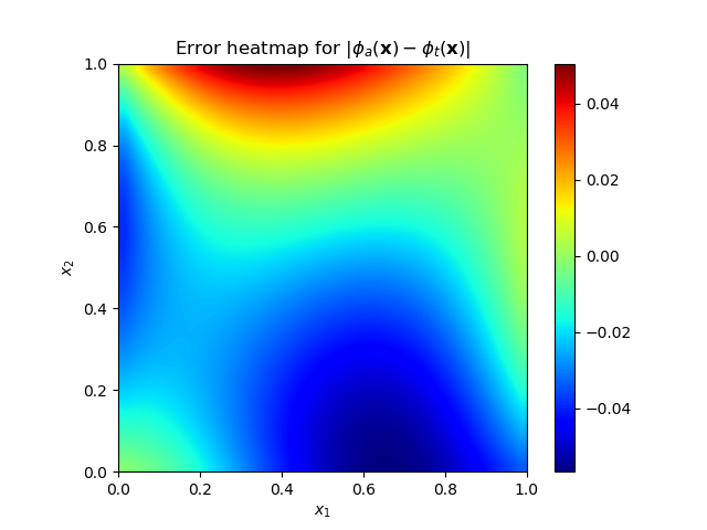 | Figure 2(a). Heat map of prediction and exact solution error |
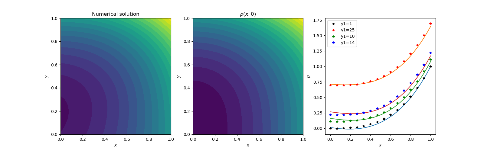 | Figure 2(b). Contour plots of exact and numerical solutions and cross section data comparison |
In conclusion, one has to be careful in using BFGS and other minimization techniques. If used wisely, it will produce better results.Case B: Our next topic will be geared towards higher dimension solution. Finite difference analysis has been attempted for three-dimensional Poisson’s equation [9]. I admire the hard work and mathematical genius of the authors. One of the test cases has the following attributes [9]:Analytical solution:u(x,y,z) = sin(𝜋x)sin( 𝜋y)sin(𝜋z)Boundary conditions:u(0,y,z) = u(1.y,z) = 0u(x,0,z) = u(x,1,z) = 0u(x,y,0) = u(x,y,1) = 0Source function (right hand side):f(x,y,z) = -3𝜋**2* sin(𝜋x)sin( 𝜋y)sin(𝜋z)For our boundary condition based neural network, it will be an easy formulation. The three-dimensional Laplacian is simply adding the third second derivative. The boundary conditions are applied to two-dimensional domain. The Adam minimization accepts any dimensional error loss. We were using sigmoid activation function for long time. We had difficulty with any zero Dirichlet boundary condition problem. A look at activation functions [10] suggested that one should use relu activation function to avoid vanishing gradient problem associated with sigmoid function. The swish activation function was chosen as it has both the relu and sigmoid properties. The following are these activation functions:Sigmoid: f(z) = 1./(1.+exp(-z))Swish: f(z) = z/(1.+exp(-z))A simple change in the activation function and their derivatives made huge difference. Our new Laplacian operator is:L(x,y,z) = δ2/δx2 + δ2/δy2 + δ2/δz2 Since there are no public domain three-dimensional plotting programs, we will show the sectional contours and the exact sectional solution in two dimensions. The computations were carried out on a 30x30x30 grid with (0,1), (0,1), (0,1) cartesian domain.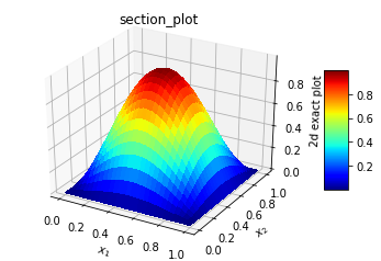 | Figure 3(a). Exact analytical solution. It is same in any two-dimensional space |
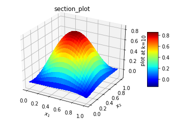 | Figure 3(b). Solution at mid z section, x-y plane |
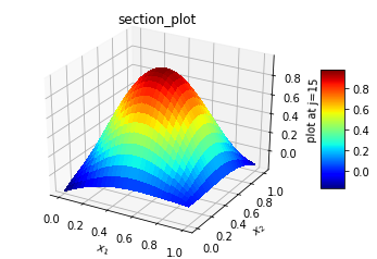 | Figure 3(c). Solution at three quarter y section, x-z plane |
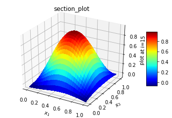 | Figure 3(d). Solution at three quarter x section, y-z plane |
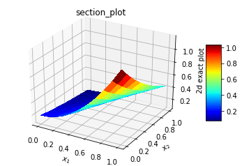
The solution involved 900 Adam optimization cycle followed by BFGS minimization. It took about 5 hours on a 8gb intel i7 personal computer. The Adam optimization had brought down loss error to 5.332e-07, so the BFGS minimization was swift in matter of seconds and error around 5.43878e-27. The L2_norm for normalized difference was 3.7284e-02. The error in L2_norm difference is quite high compared to 1.18059e-6 for 19 point and 27 point fourth order finite difference schemes [9]. Case C: Our next topic will be an extension to the fourth dimension. The formulation and setup are quick. The Laplacian is extended in fourth dimension and boundary conditions are applied to three-dimensional domain. A typical contrived test case has the following attributes:Analytical solution:u(x,y,z,t) = exp(-t)*(x**2 + y**3 + z**4)Boundary conditions:u(0,y,z,t) = exp(-t)*(y**3+z**4),u(1,y,z,t) = exp(-t)*(1 +y**3+z**4)u(x,0,z,t) = exp(-t)*(x**2+z**4)u(x,1,z,t) = exp(-t)*(1 +x**2+z**4)u(x,y,0,t) = exp(-t)*(x**2+y**3)u(x,y,1,t) = exp(-t)*(1 +x**2+y**3)u(x,y,z,0) = (x**2+y**3+z**4)u(x,y,z,1) = exp(-1)*(x**2+y**3+z**4)L(x,y,z, t) = δ2/δx2 + δ2/δy2 + δ2/δz2 + δ2/δt2 f(x,y,z,t) = exp(-t)*(2.+6.*y+12.*z**2+x**2+y**3+z**4)Due to the limited capability of computer, the solution was carried out on a 11x11x11x11 grid on (0,1) domain for 200 Adam optimization followed by BFGS minimization. It took nearly 5 hours to get the following results. The plots are presented in two-dimensional view with cuts made on a two-dimensional plane. The L2_norm for normalized difference was 1.66e-02. The results are shown below.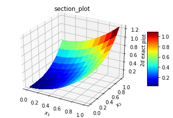 | Figure 4(a). Exact solution in x-z plane |
 | Figure 4(b). Numerical solution in x-,z plane at mid y and t section |
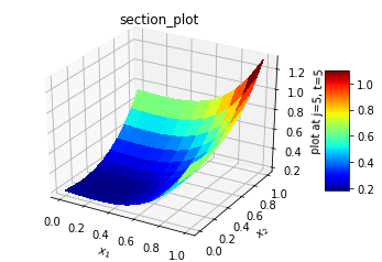
 | Figure 4(c). Numerical solution in y-z plane at mid x and t section |
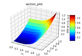
 | Figure 4(d). Numerical solution in x-t plane at mid y and z section |
 | Figure 4(e). Exact solution in in x-t plane |
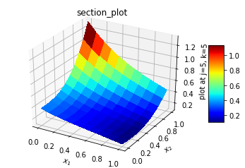
It seems like the predictions are reasonably good without any laborious finite difference derivations.Case D: The potential flow around an infinite cylinder (2D) in polar coordinate is investigated next. This is a very simple case and has been solved analytically [11]. The solution for a free stream velocity of U is given by;Velocity potential 𝛟 = U(r + 1/r)*cos(θ)The following attributes are used for this case:Laplacian L = d2 𝛟 (r, θ)/dr2 + (1/r**2)*d2 𝛟(r, θ)/d θ 2 + (1/r)*d 𝛟(r, θ)/ dr The boundary conditions used for a cylinder of radius 1, free stream velocity equal to one, and far stream boundary at radius 60 are the following;𝛟(1, θ) = 2*cos(θ), 𝛟(60, θ) = (60+(1/60))* cos(θ), 𝛟(r, -𝜋) = -(r+(1/r)), 𝛟(r, 𝜋)= = -(r+(1/r))f(r, θ) = 0The boundaries for θ are from -𝜋 to 𝜋. The obvious choice will be a range of 0 to 2𝜋. However, the solution in this range never converged. Since the neural network is cartesian in nature, a cyclic range was not very suitable. The solution is obtained on a 30x30 grid with 1000 Adam optimization cycle. It took 3172 secs to complete the analysis. The results are shown below.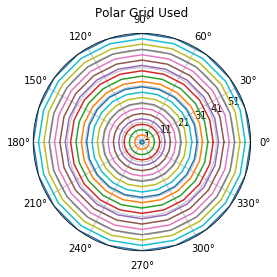 | Figure 5(a). Polar grid used. Usually known as O grid |
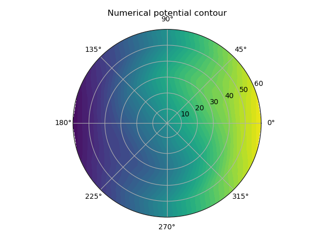 | Figure 5(b). Numerical potential color map |
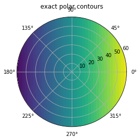 | Figure 5(c). Exact potential color map |
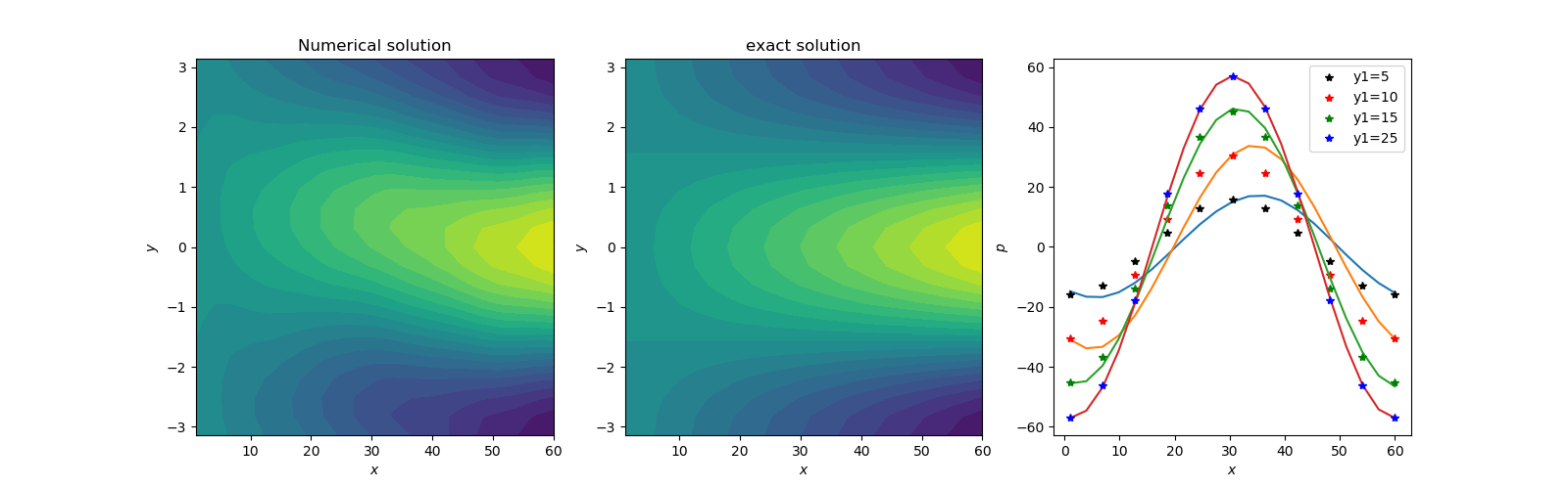 | Figure 5(d). Contour maps of potentials where x is radius, y is theta, p is potential. In the section comparison between numerical and the exact potential, y1. are the theta coordinate index |
After lots of trials, this is the best match we can get. It seems like the cartesian neural network is not very suitable for polar coordinates. We wish someone could come up with a neural network valid in arbitrary coordinate system, which will be very helpful in future applications.
3. Conclusions
The present simpler new neural network scheme with explicit boundary conditions exhibits nice capability to solve elliptic partial differential equations in low to higher dimensions with relative ease. Only proper case attributes, such as Laplacian, boundary conditions and source function, are needed. It will expedite the solution process for engineering purposes. In comparison, coming up with the finite difference or finite element schemes for 3D and 4D cases will take lots of effort and time. The error reduction still seems to be a problem with optimization and minimization schemes. The computation time in hours is too high compared to a mere few seconds with finite difference schemes. Further challenging work is needed in this area. The potential flow analysis in polar coordinates probably need better non cartesian neural network definition. The codes for all the present work are available at narain42/Poisson-s-Equation-Solver-Using-ML on GitHub.com.
References
| [1] | E. Lagaris, A. Likas, and D.I. Fotiadis, “Artificial Neural Networks for solving ordinary and partial differential equations,” arXiv:physics/9705023v1, 19th May 1977. |
| [2] | Lu Lu, “DeepXDE: A Deep Learning Library for Solving Forward and Inverse Differential Equations”, AAAI-MLPS, March 24, 2020. |
| [3] | J.P. Narain, “Solution of Poisson’s Equation Using Artificial Neural Network”, Computer Science and Engineering, Vol. 11, No. 1, June 2021. |
| [4] | Ryan Adams, “autograd”, HIPS/autograd on github.com, March 5, 2015. |
| [5] | J.P. Narain, “Efficiently Solving Poisson’s Equation Using Simple Artificial Neural Networks Computer Science and Engineering, Vol. 11, No. 2, June. |
| [6] | Luis, Angel, “Solving differential equations with neural networks,” imyoungmin/DENN on github.com, May 2, 2019. |
| [7] | Diederik P. Kingma, Jimmy Ba,” Adam: A Method for Stochastic Optimization”, arxiv, 2015. |
| [8] | SciPy, “scipy.optimize.minimize.html”, The SciPy Community, 2008-2021. |
| [9] | A. Shiferaw, and R.C. Mittal,” An efficient direct metod to solve the three dimensional Poisson’s equation”, American Journal of Computational mathematics, December 2011. |
| [10] | Vivek Patel, “Activation Functions in Deep Learning”, https://medium.com/analytics-vidhya/activation-functions-in-deep-learning-d5d7450fbd0d, 2020. |
| [11] | A.M. Keuthe and C.Y. Chow., “Foundations of Aerodyanics,”, Fifth Edition, 1998. |

 Abstract
 Reference
 Full-Text PDF
 Full-text HTML