Mečislovas Mariūnas
Department of Biomechanical Engineering, Vilnius Gediminas Technical University, Vilnius LT, Lithuania
Correspondence to: Mečislovas Mariūnas, Department of Biomechanical Engineering, Vilnius Gediminas Technical University, Vilnius LT, Lithuania.
| Email: |  |
Copyright © 2021 The Author(s). Published by Scientific & Academic Publishing.
This work is licensed under the Creative Commons Attribution International License (CC BY).
http://creativecommons.org/licenses/by/4.0/

Abstract
This paper presents method for determining mathematical model of a nonlinear two-degree-of-freedom dynamic system. It has been found that the mathematical model of a nonlinear dynamic system with two degrees of freedom can be described by 9 second-order linear differential equations, which are obtained in some way by combining subsystem differential equations based on resonant and parametric frequency. However, it is emphasized that in order to create a proper dynamic mathematical model of a system, it is necessary, in addition to proper determination of its parameters, excitation forces and parametric vibration frequencies, to evaluate also the constraints assigned to this system. The dependence of the magnitude of the amplitudes of the parametric excitation forces on the change of its frequency was determined and the relationship between their number and the nonlinearity of the dynamic system was explained. Methods of creating excitation force matrices and their properties are analyzed as well. It was found that the number of columns of the excitation force matrix, i.e. the length of the rows, depends on the degree of nonlinearity of the dynamic system. The certainty of the analytical methods presented in the paper was verified by numerical calculations.
Keywords:
Method for determination mathematical model, Two degree of freedom, Excitation forces, Dynamic system, Quadratic, Cubic and fourth order nonlinearities, Vibration, Eigenvalues, Parametric excitation force
Cite this paper: Mečislovas Mariūnas, Method for Determining a Research Model of Nonlinear Two Degree of Freedom Dynamic System, American Journal of Computational and Applied Mathematics , Vol. 11 No. 1, 2021, pp. 1-11. doi: 10.5923/j.ajcam.20211101.01.
1. Introduction
In order to create a nonlinear mechanical dynamic system and ensure its sustained and stable operation, safe working conditions need to be determined. This can be done only by creating a mathematical model suitable for the (assigned) chosen nonlinear dynamic system parameters and creating a solution method that would allow minimizing the vibration level of the designed dynamic system. The mathematical model of a nonlinear dynamic system can be formed according to D’Alembert’s principle, Lagrange, Virtual work methods or in other ways. However, an exact method for solving the equations of the constructed mathematical model has not yet been created and various approximate methods and numerical calculation methods are applied for its solution. In this paper, the example of two degree of freedom coupled oscillator with quadratic, cubic and fourth order nonlinearities stiffness is considered. This system is representative of a range of applications in structural dynamics, see [1- 13]. In [1], the measure theory is applied to solve a wide range of second-order boundary value ordinary differential equations. First, they transform the problem to a first order system of ordinary differential equations (ODE’s) and then define an optimization problem related to it. To solve this problem in the work [2], the authors applied three different approximate solution methods: variation of parameters, differential transformation, and Adam's decomposition. In order to compare properly the accuracy and efficiency of the method of variation of parameters to the semi-analytical methods, all three methods were implemented in MATLAB. Thus, they used the results of the numerical method to estimate the accuracy of the approximate method. In [3], three iterative methods have been implemented to solve several second order nonlinear ODEs arising in physics. The obtained results were compared numerically with other numerical methods. The results of the maximum error remainder values show the present methods to be effective and reliable. Thus, and they used the results of the numerical method to estimate the accuracy of the approximate method. For example, the method of multiple scales perturbation technique used in [7-8] to analyze the response of this system. Four ordinary differential equations are derived to describe the modulation of the amplitudes and phases of the two modes of vibrations for the principal parametric resonances. The steady-state solutions and their stability are determined and representative numerical results are included. The theoretical resonance cases of this system have been obtained from the first approximation differential equations and some of them are confirmed by applying well-known numerical technique. The stability of the obtained numerical solution is studied using phase–plane method. The effects of different parameters on the vibration of this system are investigated [5]. In this study, they provide an analytical method for relating the backbone curves, found upon using the second-order normal form technique, to the forced responses. This is achieved upon applying an energy-based analysis to predict the resonant crossing points between the forced responses and the backbone curves. In addition, a method for assessing the accuracy of the prediction of the resonant crossing points is then introduced, and these predictions are then compared to responses found using numerical continuation. In [9], the vibration of a typical two degree of freedom nonlinear system with repeated linearized natural frequencies was systematically investigated. The method of multiple scales is used to obtain the amplitude-phase portraits by introducing the energy ratios and phase differences. It is found that the normal in-unison modal motions, elliptic out-of-unison modal motions are analogous to the polarization of classical optic theory. Further, some kinds of periodic and chaotic motions under out-of-unison and in-unison excitations are investigated numerically. The result of that study offers a detailed discussion of nonlinear modal motions and responses of two degree of freedom systems with cubic nonlinear terms.In [11], the amplitude frequency characteristic equation of the system, based on the multi-harmonic method, and the corresponding curve of the relationship between the amplitude and frequency is derived. The influence of the current on the curve is researched as well. The results showed an existence of two pseudo-resonant peaks in the amplitude–frequency curve; one of them is in the low frequency band, and the other – in higher frequency band. The one of the most helpful approximation methods, namely, the expansion of a solution of a differential equation in a series in powers of a small parameter was used in [12]. They used the Lindstedt-Poincaré perturbation method to construct a solution closer to uniformly valid asymptotic expansions for periodic solutions of second-order nonlinear differential equations. In [3-4,7-9], approximate methods and numerical research have also been applied in research to investigate nonlinear dynamical systems. However, the results of the nonlinear two degree of freedom system determined in this way are not accurate enough, and an analysis of the literature shows that there is no accurate and clear analytical way to determine the level of dynamic system vibrations under the action of external forces. In short, the applied approximate methods do not explain the physics of vibration of nonlinear dynamical systems. Moreover, they do not show the specificity of their behavior compared to linear systems. The resonant and parametric frequencies in nonlinear one and two degree of freedom dynamic system were analyzed [6,13]. That paper presents methods for determining resonant and parametric excitation frequencies in a nonlinear one and two-degree-of-freedom dynamic systems. It was clarified that a nonlinear dynamic system or subsystems has four resonant frequencies, which are defined by the characteristics of the energy, force, and stiffness connection peculiarities, as well as the total stiffness of the subsystems. The results also demonstrate that the system or subsystems generates a very wide spectrum of parametric excitation frequencies. However, analytical methods are developed only to determine the frequencies of nonlinear dynamical system resonant and parametric vibrations and the problem of its mathematical modeling was not considered. Therefore, in the design stage of a dynamic system, it is very important to create a mathematical model that, by considering the resonant, parametric and external excitation frequencies of the system, would allow reducing its vibration level and ensure safe working conditions. Thus, the purpose of the research was to study the vibrations of nonlinear two-degree-of-freedom dynamic systems, to explain their features, to provide methods for creating a mathematical model, determining the resonant and parametric excitation frequencies of the system, to clarify and determine the forces acting on the system during operation, generated through the properties of the nonlinear dynamic system itself, and to show their destructive effects on the vibration level of the system.
2. Method for Determining Research Model of Nonlinear Two-Degree-of-Freedom Dynamic System
Nonlinear two-degree-of-freedom dynamic system vibrations (Figure 1) in [6] are described by the following system of equations: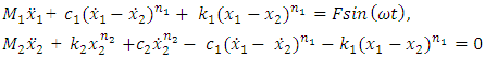 | (1) |
where  are masses of the system;
  are coefficient of damping;
  are coefficient of stiffness;
  are exponents of
 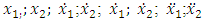 are velocity and acceleration; F is amplitude of external excitement force;
  is angular frequency; t is time.
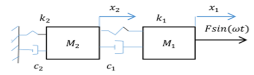 | Figure 1. Two degree of freedom vibration system for linear motion |
The system of equations (1) in [6] was divided into two subsystems. Four differential equations were formed for each of them (see (4) and (8) in [6]), which allow to determine the resonant frequencies of those subsystems: for the first subsystem 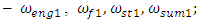 for the second subsystem
 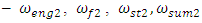 and the frequency
  , which is generated by the total stiffness of the system. In this way, 9 resonant frequencies (eigenvalues) were determined in both subsystems, on the basis of which nine second-order differential equations can be formed. In order to create a mathematical model of a dynamic system from the available nine equations, it is necessary to combine them all into one system. Using the method of partitioning a system of equations into separate subsystems and combining them into a common system used [6], 9 second-order differential equations are combined into one system:
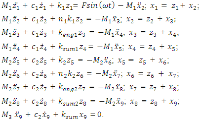 | (2) |
Upon expressing the dependences of  and
and  from the variables of the connection equations given for each differential equation in the system (2) and inserting into the corresponding differential equations we obtain in matrix form:
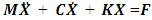 | (3) |
where M is a mass matrix; C is the matrix of damping coefficients; K is the stiffness matrix;  and
and  are columns of acceleration, velocity, and displacement vectors; F is a matrix of forces acting on a dynamic system, the expressions of which are given in (14) and (15).The damping coefficient and stiffness matrices are shown below:
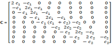 | (4) |
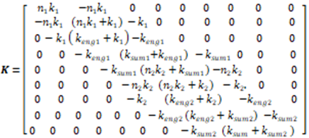 | (5) |
The mass matrix M is a square 9x9 dimension whose basic diagonal elements are: 

 and all other elements have values of zero. In this way, the systems of left equations (3) are clear because the matrices of mass, damping coefficient (4) and stiffness (5) are known. However, in order to determine the matrix F of forces acting on the system, additional studies are required. It is very important to make sure how much the resonant frequencies (eigenvalues) will change when the latter subsystems are combined into a common system. For the determination of eigenvalues, the system of equations (3) is rearranged as follows:
  | (6) |
The system (6) can be solved by guessing the solution:  . By inserting
  in to the system (6) and denoting
  we obtain:
 | (7) |
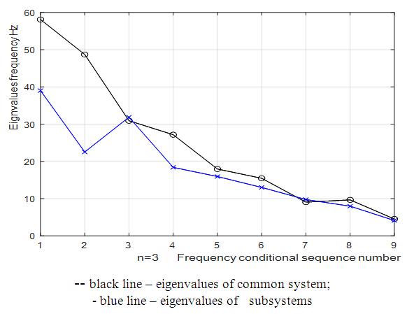
In order to determine the influence of excitation force frequency, parametric and resonant frequencies on the magnitude of nonlinear dynamic system vibrations, let us conceder their relationship in a simplified diagram in Figure 3. For this purpose, a system of equations (7) was solved using MATLAB, the result of which and the resonant frequency graph of the subsystems are shown in Figure 2. When examining the results of the Figure 2 graphs, that is, comparing them, it is necessary to note that the curves are shifted with respect to each other. In the upper part of the diagram of Figure 3, the resonant frequencies 
 which are arranged in ascending order are relatively displayed.
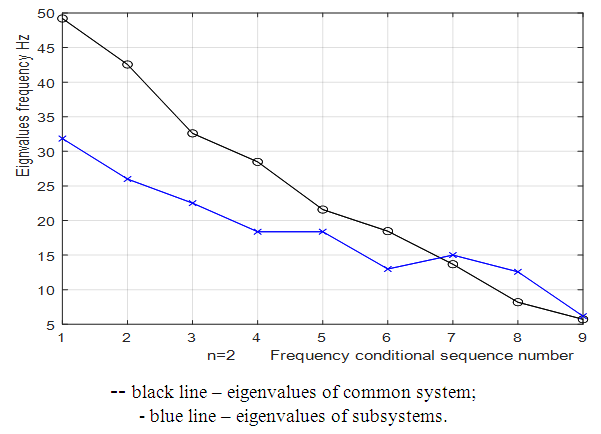 | Figure 2. Eigenvalues for the system with quadratic nonlinearity, when  = 40000 N/m; = 40000 N/m;  = 100000 N/m; F = 100000 N; = 100000 N/m; F = 100000 N;  = 5.0 kg; = 5.0 kg;  = 3.0 kg and c = 0.05 = 3.0 kg and c = 0.05 |
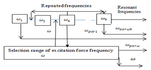 | Figure 3. Simplified connection scheme of external excitation, resonant and parametric frequencies |
In the lower part of the considered scheme, the range of allowable variation of the external excitation force frequency  is relatively shown. On examining the connections between frequencies of external forces, parametric vibrations and resonant frequencies in the simplified scheme presented in Figure 3, we can observe that there are three characteristic cases: 1 – when
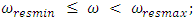
 and
and  Values of
  and
and  are determined as follows:
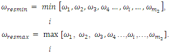 | (8) |
where  is the number of resonant frequencies;
  when
when  are the resonant frequencies of a nonlinear dynamic system.We will consider bellow each of the three possible connection peculiarities listed above between frequencies of external forces, parametric vibrations, and repetitive frequencies. The first case when
 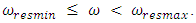 For this case, the relationships between external excitation forces, parametric vibration, and resonant frequencies are shown in a simplified manner in Figure 3. Thus, if we randomly choose the external excitation frequency
  , which is equal to
  , then, in addition to vibrations of the latter resonant frequency, repetitive frequency vibrations may occur in the system. We will say that
  and
and  are repetitive frequencies of the excitation force frequency. Thus, in the simplified nonlinear dynamic system presented in Figure 3, in addition to the external excitation force frequency, parametric vibration frequencies can be generated, thus there would be three more parametric vibration excitation frequencies
 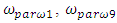 and
and  By changing the dynamic parameters of the nonlinear system and the frequency of external excitation force, it is possible to try avoiding repetitive resonant frequency to the external excitation frequency and reducing the vibration level in the system. However, if there are any constraints, then the latter problem becomes more difficult and in fact nonlinear programming problems need to be solved with linear constraints. In this case, by creating a mathematical model of a nonlinear dynamical system, we should solve the latter problem and get the only optimal variant for it. However, using the method of analysis and evaluating the restrictions, we can approximately determine the parameters of the dynamic system and the external excitation force frequency, which would allow to reduce the vibrations level of the dynamic system and would enable ensure sufficiently good working conditions. Let us consider how to determine the magnitude of the parametric excitation force generated by a dynamic system.In [6] it was shown that the forces generating parametric vibrations are in fact forces of a kinematical excitation nature, the magnitude of which can be determined as follows:
 | (9) |
where  is the mass vibrating at the resonant frequency,
  is the amplitude of the resonant frequency vibrating masses;
  is the resonant frequency at which the mass
  is vibrated.In [6], the value of the parameter
  is determined as follows:
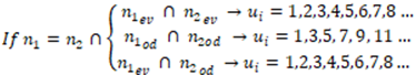 | (10) |
where  and
and  are even numbers;
  and
and  – odd numbers;
  is conjunction;
  is implication;
  are exponents of
  and
and  (see (1));
  is the number of the harmonic sequence of the parametric vibrations.The expression of the ratio amplitudes of the parametric forces of
  and
and  will be as follows:
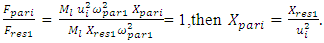 | (11) |
In this case, when the system will be resonant, the magnitude of amplitude is calculated upon applying the following formula: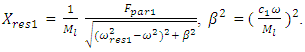 | (12) |
It can be seen from (11) and (12) that the amplitude of the vibration  in the case of resonance is
  times smaller than the amplitude of vibration
  excited by the excitation force, which means that
  must also be
  times smaller than
  . In this way, the magnitudes of the harmonic amplitude of the excitation forces of the parametric vibrations can be determined as follows:
 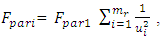 | (13) |
where  is the number of parametric excitation force harmonics.Let's examine the content of the excitation force matrix when
  that is, the amplitude of the last excitation force harmonic would be 25 times smaller. It is stated that in the considered scheme (Figure 3), the external excitation force acts on the first subsystem with mass
  Therefore, its effect must be estimated by the equation on the right side of the fourth equation of the system (3). In the first subsystem, the force generated by the amplitude of the first resonance excites vibrations at a frequency of 31.85 Hz, and we will evaluate its effect on the right side of the first equation. The force generated by the amplitudes of the second resonance acts on the second subsystem with mass 𝑀2. Thus, the latter force in the system of equations (3) must be evaluated on the right-hand side of the 8 equation. When
  and
and  are even numbers, then the excitation force matrix F is of the form (14). When n is an odd number then the excitation force matrix
  is of the form (15).
 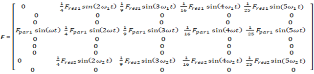 | (14) |
In a linear dynamic system, vibrations of repeated resonant frequencies are also excited, but the harmonics of parametric vibrations will not be excited. Therefore, when constructing the excitation force matrices (14) and (15), we must evaluate that property. This means that the value of the first term in the rows of repetitive frequency parametric forces will be zero (see (14) and (15)). It can be seen from matrices (14) and (15) that in order to achieve the same results for accuracy, the number of columns in the latter force matrices should not be the same. If the external excitation frequency changes or the nonlinear dynamic system parameter values change, then the structure of matrices (14) and (15) and the values of their elements change as well. It follows that in order to reduce the nonlinear system vibration level, the external excitation force frequency and system parameter values cannot be randomly chosen. This means that the interaction between the external excitation force frequency and the system parameters must be matched in each case to ensure a minimum system vibration level. In other words, an acceptable mathematical model of a nonlinear dynamic system can be developed for each case using a simplified method of synthesis analysis.The second case, when  and the third case, when
  , can be interpreted in a similar way as the first case. Therefore, we will not stay on their interpretation.
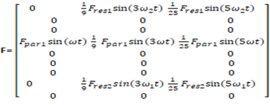 | (15) |
The analysis of (2 - 13) the dependencies, as well as the data provided in matrix (14), (15) and Figure 3 shows that in order to create a mathematical model of nonlinear dynamical systems it is necessary to perform mathematical and logical operations in the following order: 1. We assume nonlinear dynamic system parameters namely: masses, spring stiffness, damping coefficients and system nonlinearity indices; 2. Upon applying the D’Alembert’s principle or Lagrange or Virtual Work methods, we determined a mathematical model of a nonlinear dynamic system;3. The system of nonlinear dynamic model is divided into subsystems according to the methodology presented in [6] and the resonant frequencies (eigenvalues) of the subsystems are determined.4. Dynamic subsystem resonant frequency analysis is performed. If it is found to have the same frequency or repetitive frequency then you need to change the nonlinear dynamic system parameter magnitudes you have chosen or assigned to you. Sometimes it may be enough to change the magnitudes of only a few parameters and it will be possible to avoid the same magnitude or repeated frequencies in the system.5. According to the previously analyzed methodology, the frequencies of nonlinear dynamical system parametric frequencies are determined and an excitation force matrix (14) or (15) is formed. 6. If the same or repeated frequencies occur between the resonant and parametric frequencies of the system, then the external excitation force frequency could be changed. If this is not possible then the magnitude of the nonlinear dynamic system parameters should be changed. This means that it is necessary to repeat the calculations from the first position and choose other nonlinear dynamic system parameters when analyzing the calculation results. 7. The cycle of simplified analysis synthesis is repeated until an acceptable mathematical model of the nonlinear dynamical system is created.Thus, the analysis demonstrates that using simplified synthesis analysis methods, a nonlinear dynamical system can be described as a linear system of second - order differential equations and its acceptable mathematical model can be created.
3. Numerical Analysis and Discussion
In order to compare the resonant frequencies (eigenvalues) of the common system and subsystems, calculations of the latter subsystems were performed using MATLAB. The resonant frequencies of the nonlinear dynamic system with the quadratic nonlinearity, whose the system parameters are:  = 100000 N/m;
  = 40000 N/m; F = 100000 N;
  = 5.0 kg;
  = 3.0 kg;
  = 0.05, were calculated using formulas (5), (7-11) presented in paper [6]. The following results were obtained:
  = 18.39 Hz;
  = 22.52 Hz;
  = 31.85 Hz;
  = 12.99 Hz;
  = 15.01 Hz;
  = 18.38 Hz;
  = 26.00 Hz;
  = 12.59 Hz;
  = 6.17 Hz. In order to compare the calculated eigenvalues according to (7) dependences with the resonant frequencies of the dynamic system of cubic nonlinearity, their values also were determined. For the system with cubic nonlinearity whose parameters are:
  = 100000 N/m;
  = 40000 N/m;
  = 100000 N;
  = 5.0 kg;
  = 3.0 kg;
  = 0.05, the resonant frequencies of the system are:
  = 15.92 Hz;
  = 22.52 Hz;
  = 39.00 Hz;
  = 9.75 Hz;
  = 13.00 Hz;
  = 18.39 Hz;
  = 31.85 Hz;
  = 7.96 Hz;
  = 4.12 Hz. The initial data of the parameters for the dynamic system are usually given a priori, but their sizes can be changed during the modeling process.Resonant frequencies and eigenvalues of quadratic and cubic nonlinearity dynamical systems calculated with the help of MATLAB are shown in Figures 2 and 4. The latter results show that in the common quadratic nonlinearity system, two frequencies of 49.21 and 42.56 Hz occur, and in the cubic nonlinearity system, frequencies of 58.10 and 48.69 Hz occur, which were not present in the spectra of the subsystems. The other frequencies of the quadratic and cubic nonlinearity systems overlap or are close to the frequencies of the subsystems. The results of the calculation according to the system of equations (3) when the excitation force frequency
  = 35 Hz is not equal to the resonant frequency of the quadratic nonlinear system are shown in Table 1 below. The latter result shows, firstly, that the vibration levels are not the same for the individual coordinates or for the different resonant frequencies of the system, and secondly, their analysis makes it possible to identify the resonant frequencies with the highest vibration levels and make appropriate decisions. The results provided in the Table 2 show that when the excitation force frequency is of the same magnitude as the resonant frequency of the system, then the level of vibrations of almost all resonant frequencies of the system increases significantly. Very high vibrations according to the coordinates
  and
and  , which correspond to the resonant frequencies of the system f = 12.59 and 18.38 Hz (Figure 2), are due to the fact that their frequencies are repeated of the external excitation force frequency f = 6.17 Hz. Figure 5a shows all 5 components of the parametric vibration and the resonant frequency of the f = 49.85 Hz system.
 Table 1. The magnitude of linear dynamic system’s vibrations by individual coordinates in the case of non-resonance, f = 35 Hz
 |
| |
|
Table 2. The magnitude of linear dynamic system‘s vibrations according to individual coordinates in the case of resonance, f = 6.17 Hz
 |
| |
|
 | Figure 4. Eigenvalues for the system with cubic nonlinearity when  = 40000 N/m; = 40000 N/m;  = 100000 N/m; = 100000 N/m;  = 5.0 kg; = 5.0 kg;  = 3.0 kg = 3.0 kg |
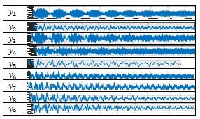
Meanwhile, in Figure 5b, all components of the parametric vibrations and the resonant frequency of the system, f = 49.85 Hz, are not visible due to the very increased level of vibrations at f = 6.17 Hz. Using the same system parameters as in the calculation of the linear system vibrations, the non-linear system vibration level characteristic parameters are calculated, some of which are shown in Figure 6 below. Comparing the results calculated according to a linear mathematical model with the results calculated according to the nonlinear model, we will observe that in the case of resonance in the linear system the maximum vibration level is  (Table 2), and in the nonlinear system (Figure 6a) –
  . In a linear and nonlinear dynamic system, very low frequency vibration waves occur, the frequency of which is: in the nonlinear system in the range of about 2.1 Hz and 0.65 - 0.76 Hz, and in the linear system - in the range of about 3Hz and 0.31 - 0.33 Hz. The frequencies of their vibration spectral densities are practically the same, but some of them have different intensities, especially the resonant frequency which coincides with or is a repeated of the external excitation force frequency. Thus, the calculation results according to (3) performed using MATLAB showed that in the linear dynamic system the maximum vibration magnitude excited by resonant frequencies is about 8.63 times higher than in the quadratic nonlinearity system and approximately the 34.17 time as in the non-resonant linear system state. Meanwhile, in a nonlinear dynamic system, when the vibration is excited with a resonant frequency
  = 13.68 Hz, the maximum vibration amplitude is
  and when it is excited with a non-resonant frequency then
  Thus, in the non-resonant case, in a system of quadratic nonlinearity, the vibration intensity decreases by about 4.20 times.
 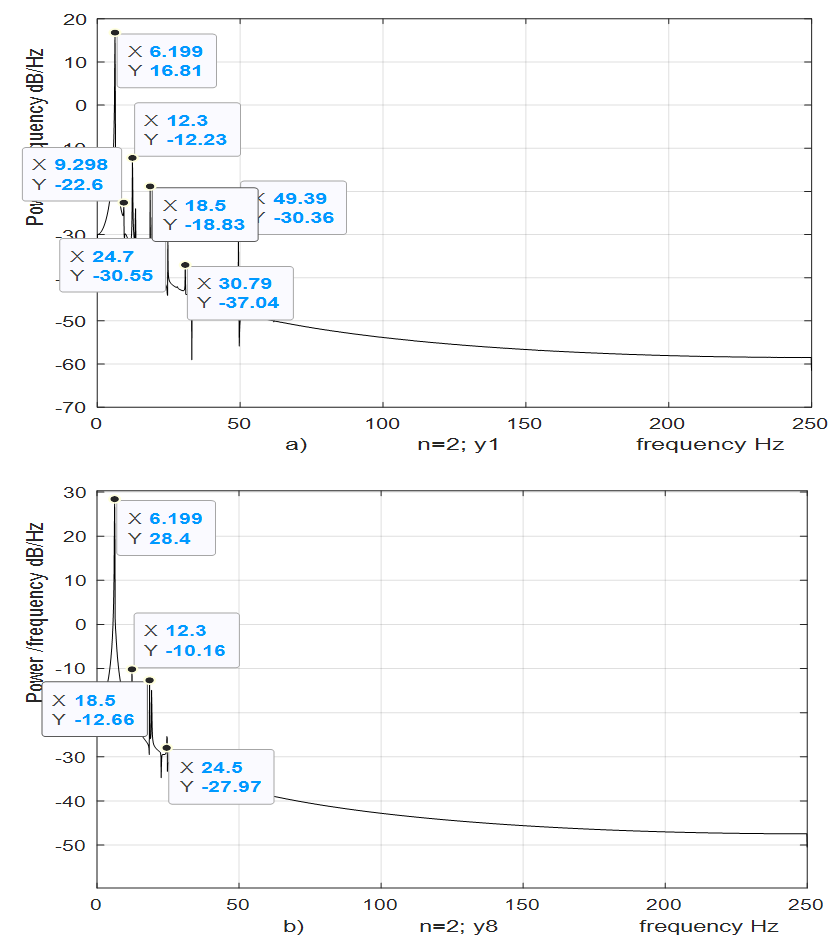 | Figure 5. Result of solution of spectral density for the quadratic nonlinearity when  = 40000 N/m; = 40000 N/m;  = 100000 N/m; = 100000 N/m; 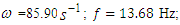 F = 100000 N; F = 100000 N;  = 5.0 kg; = 5.0 kg;  = 3.0 kg and = 3.0 kg and  |
 | Figure 6. Result of solution of vibration and spectral density for the quadratic nonlinearity when  = 40000 N/m; = 40000 N/m;  = 100000 N/m; = 100000 N/m;  ; ;  F = 100000 N; F = 100000 N;  = 5.0 kg; = 5.0 kg;  = 3.0 kg and = 3.0 kg and  |
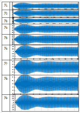
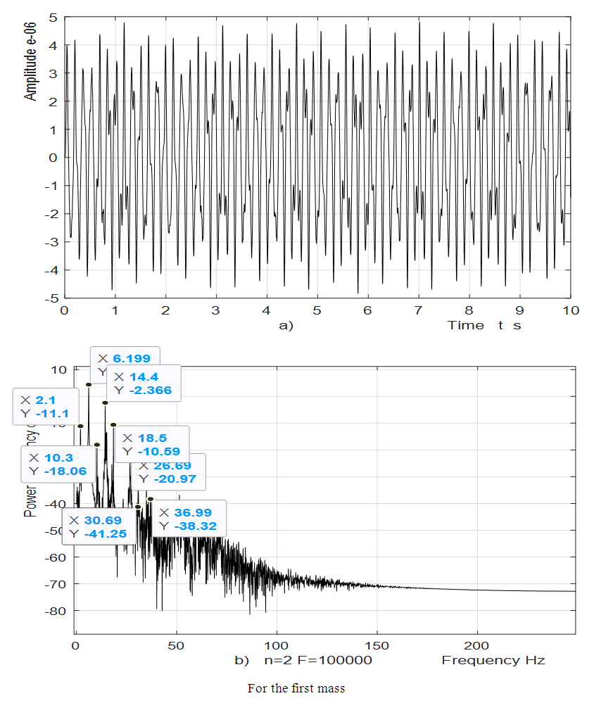
For cubic and fourth-order nonlinearity dynamical systems, analogous studies were performed as for the quadratic nonlinear dynamics system. However, their full results cannot be provided due to the limited size of the paper. Therefore, Figures 7 and 8 below show only a part of the research result calculated by linear and nonlinear mathematical models for cubic nonlinearity systems. Figures 7b and 8c show that when the system is excited at a system resonant frequency of 13.40 Hz, the spectrum of the first mass has lower frequencies, including 4.08 Hz. However, when a nonlinear system is excited by a higher force in Figure 8b, then the lower frequency spectrum is not visible because their vibrations are offset by intense vibrations at the higher frequencies. It should be noted that in the process of studying the dynamic system linear model, only the parametric vibrations generated by the excitation force were evaluated. Comparing the results calculated according to the linear mathematical model with the results calculated according to the nonlinear model, it is observed that in the case of resonance in the linear system of cubic nonlinearity, the maximum vibration level is  and in the nonlinear -
 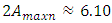 . Hence, in this case, the magnitudes of the maximum vibration differ about 2.16 times only. Thus, the above comparative analysis of the maximum vibrations shows that the nonlinear dynamic system damped the vibrations more than the linear system. And this property of nonlinear dynamical systems can be explained by the resonant conditions in them, namely, that the resonant conditions in the system exist only if 1- ε ≤ x ≤ 1+ ε within those limits (where ε magnitude is small enough, see [6]). The results of further research, especially on the vibration damping properties in a nonlinear dynamic system, will allow to refining (improve) the mathematical model presented in this paper. In the case of cubic and fourth-order nonlinearity in dynamic systems, vibration waves with a lower frequency than vibration waves of the resonant frequency of the system are also observed. Therefore, the results of the study showed that dynamic systems of cubic nonlinearity are more robust (more stable) than dynamic systems of quadratic nonlinearity. Thus, the results of the study show that it is necessary to determine the parameters and external excitation force frequencies of the nonlinear dynamic system that would guarantee non-resonant operating conditions. Thus, the advantage of the developed linear model of a nonlinear dynamic system compared to approximate methods is that it allows: to understand the ongoing processes in a dynamic system; to determine the frequencies of resonant and parametric vibration and the forces generated by parametric vibrations, taking into account the level of nonlinearity of the dynamic system, on the basis of which the mathematical model is formed, and to select appropriate system parameters and operating modes. In addition, the developed mathematical model of the dynamic system enables analyzing the system vibrations and their intensity in each resonant and parametric vibration frequency and by changing the dynamic system parameters to reduce their detrimental effect on the qualitative properties of the object. Meanwhile, various approximate methods do not allow understanding the ongoing phenomenon in a nonlinear dynamic system, in which a mathematical model is formed intuitively, which only approximately determines not all resonant and parametric vibration frequencies of the system and only approximate system parameter values and operating modes. Notwithstanding [1-13], such results have not been reported and no analytical study of the relationships between resonant and parametric frequencies has been performed and their connection with the mathematical model of the dynamic system has not been performed. Moreover, scientific works [1-13] do not reveal: force, stiffness and energy relations in the vibrating nonlinear dynamical system and their influence on mathematical model. In this way, it was impossible to explain the physics of the processes taking place in the vibration nonlinear dynamic system, to create a nonlinear mechanical dynamic system and to determine its safe working conditions, which ensure its long-lasting and stable operation. The numerical investigation showed that the presented methods for determining the mathematical model may be applicable in the design process of nonlinear dynamic systems for quadratic, cubic and fourth order nonlinearities of the two-degree-of-freedom system.
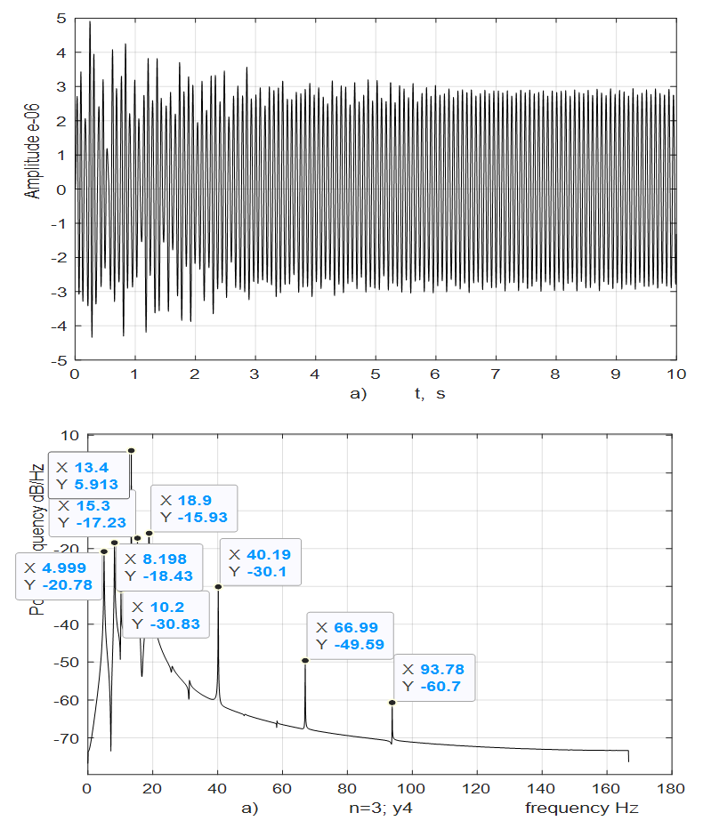 | Figure 7. Result of solution of vibration and spectral density for the cubic nonlinearity, according to the formed linear mathematical model, when  = 40000 N/m; = 40000 N/m;  = 100000 N/m; = 100000 N/m;  F = 100000 N; F = 100000 N;  = 5.0 kg; = 5.0 kg;  = 3.0 kg and = 3.0 kg and  |
 | Figure 8. Result of solution of vibration and spectral density for the cubic nonlinearity, according to the nonlinear mathematical model, when  = 40000 N/m; = 40000 N/m;  = 100000 N/m; = 100000 N/m;   = 5.0 kg; = 5.0 kg;  = 3.0 kg and = 3.0 kg and  |
4. Conclusions
This paper presents analytical method for determining the mathematical model of the systems, which enables choosing reasonable dynamic parameters of the system during the design process for quadratic, cubic and fourth order nonlinearities of two-degree-of-freedom nonlinear systems and to reduce its vibration level.Analytical results The analytical results indicate that:1. To create a linear mathematical model of a nonlinear dynamic system, it is necessary to determine the frequency of subsystems resonant and parametric vibrations;2. It is shown that for the resonant frequencies determined by the dynamic subsystem, 9 independent second order linear differential equations are formed, which are combined into one system to form a linear mathematical model of the nonlinear system.3. The dependence of the magnitude of the amplitudes of the parametric excitation forces on the change of its frequency was determined and the relationship between their number and the nonlinearity of the dynamic system was explained.4. In order to avoid the coincidence of the external excitation force frequency with the resonant frequency of the subsystems, as well as to avoid the same resonant frequency in the system, it is necessary to determine the dynamic system parameters and frequency of external excitation force by a simplified analysis-synthesis method.The results of numerical calculationsThe results of numerical calculations allow us to prove that:1. The studies have shown that models of linear and nonlinear dynamical systems have the same resonant frequencies (eigenvalues). The developed models of dynamic systems enable determining the intensity of vibrations at the resonant frequency of each system, as well as the repetitive frequencies.2. In addition to the determining the resonant frequency of the system, it also contains subharmonics of lower frequencies.3. The certainty of the analytical methods was verified by numerical calculations.
References
| [1] | Effati S., Kamya A. V., Farahi M. H., 200, A new method for the solving the nonlinear second – odder boundary value differential equations. Korean Journal of Computational and Applied Mathematics, volume 7, pp. 183 -193. |
| [2] | Travis J. More, Vedat S. Erturk, 2019, Comparison of the method of variation of parameters to semi-analytical methods for solving nonlinear boundary value problems in engineering. Nonlinear Engineering, Volume 9, Issue 1, pp. 1 – 13. |
| [3] | Al-Jawary M. A., Adwan M. I., Radhi G. H., 2020, Three iterative methods for solving second order nonlinear ODEs arising in physics. Journal of King Saud University. Volume 32, Issue 1, pp. 312-323. |
| [4] | Richard h. Rand, 2005, Lecture Notes on Nonlinear Vibrations. Depart. Theoretical and Applied Mechanics. Cornel University, Ithaca N.Y., 14853, rhr2@cornell.edu, p. 111, http://www.tam.cornell.edu/randdors/. |
| [5] | Fereidoon A., Ghadimi M., Barari A., Kaliji H. D. and Domairry G, 2012, Nonlinear vibration of oscillation systems using frequency – amplitude formulation. Shock and Vibration, 19, pp. 323-332. |
| [6] | Mariūnas M., 2020, Methods for Determining Resonant and Parametric Excitation Frequencies of Nonlinear Two Degree of Freedom Dynamic Systems. American Journal of Computational and Applied Mathematics, 10(2), pp. 39-47. |
| [7] | Goge D., Sinapius M., Fullekrug U., M. Link M, 2005, Detection and description of non-linear phenomena in experimental modal analysis via linearity plots, International Journal of Non-linear Mechanics, 40, pp. 27-48. |
| [8] | Peng Z. K., Lang Z. Q., and Billings S. A, 2006, Resonances and Resonant Frequencies for a Class of Nonlinear Systems. Department of Automatic Control and Systems Engineering. University of Sheffield. Research Report No. 920, p. 30. |
| [9] | Ji, J. C., Li, X. Y., Zhang. L. Z, 2012, Two–to–one resonant Hopf bifurcation in a quadratic nonlinear oscillator involving time delay. Bifurc. Chaos 22, pp. 1-14. |
| [10] | Luo J., Liu X, 2015, An approximate response of the large system with local cubic nonlinearities subjected to harmonic excitation. Engineering review, Vol. 35, Issue 1, pp. 49-59. |
| [11] | Bhrawy A. H., . Abd-Elhameed W. M., 2011, New Algorithm for the Numerical Solutions of Nonlinear Third-Order Differential Equations Using Jacobi-Gauss Collocation Method. Mathematical Problems in Engineering Volume 2011, p. 14. |
| [12] | Safia Meftah, 2018, A New Approach to Approximate Solutions for Nonlinear Differential Equation. International Journal of Mathematics and Mathematical Sciences. Volume 2018, p. 8. |
| [13] | Mariūnas M., 2020, Methods for Determining Resonant and Parametric Excitation Frequencies of Nonlinear One Degree of Freedom Dynamic Systems. American Journal of Computational and Applied Mathematics, 10(1), pp. 6-14. |

 Abstract
 Reference
 Full-Text PDF
 Full-text HTML