Janeth J. Ngana1, Livingstone S. Luboobi2, Okelo J. Abonyo3
1Pan African University, Institute for Basic Sciences, Technology and Innovation, Nairobi, Kenya
2Strathmore University, Nairobi, Kenya
3Jomo Kenyatta University of Agriculture & Technology, Nairobi, Kenya
Correspondence to: Janeth J. Ngana, Pan African University, Institute for Basic Sciences, Technology and Innovation, Nairobi, Kenya.
| Email: |  |
Copyright © 2019 The Author(s). Published by Scientific & Academic Publishing.
This work is licensed under the Creative Commons Attribution International License (CC BY).
http://creativecommons.org/licenses/by/4.0/

Abstract
Very few ecological studies have modeled Population Dynamics of the Serengeti Ecosystem. This paper seeks to analyze and forecast the trends of the Population Dynamics of the migratory ungulates of the Serengeti Ecosystem, under normal conditions. To get the Population Dynamics, we formulated a model of the four Ordinary Differential Equations for: Vegetation biomass, Herbivores, Lions and Cheetahs. For analysis we used the Least Mean Square method to simulate the model. We found that as the Vegetation biomass increases, the Herbivores population also increases and as a result the population of the Lions increases and the small Cheetah population decreases and goes to extinct due to competition with the Lions.
Keywords:
Cheetahs, Herbivores, Lions, Population dynamics, Serengeti ecosystem, Vegetation biomass
Cite this paper: Janeth J. Ngana, Livingstone S. Luboobi, Okelo J. Abonyo, Mathematical Model for the Serengeti Ecosystem under Normal Climate Conditions, American Journal of Computational and Applied Mathematics , Vol. 9 No. 4, 2019, pp. 97-101. doi: 10.5923/j.ajcam.20190904.01.
1. Introduction
The existence of Wildebeest, Zebra and Thomson’s gazelles in the Serengeti is very important both ecologically and economically. Ecologically, they play a vital role in ecosystem function and provide a number of ecosystem services (Bedelian, 2014). They also have a direct effect on predator populations and other wildlife species, and on grass food resources (Sinclair et al., 2008). Economically, the ungulates are important because they draw tourism and thus contribute significantly to the national economy.Declining ungulates population within national parks and wildlife reserve have become an object of growing concern with regard to the preservation of Africa’s rich large mammals diversity (Caro & Scholte, 2007), especially in the case of migratory populations (Harris et al., 2009; Owen-Smith & Ogutu, 2012).Ngana et al. (2014) did a research on the modeling of the population dynamics and the Great Migration of the Serengeti ecosystem. They used a prey-predator model and the migration equation to get the ODE’s of the Grass, Herbivores and the Lions and Crocodiles, and did a simulation to get the population dynamics, without impact of climate change on the population dynamics. The result was that the Herbivores population was increasing, as well as the Carnivores population. In this paper, we consider the dynamics of the Serengeti Ecosystem under normal conditions. We formulate a Predator-Prey Model consisting four Ordinary Differential Equations for the interaction between, Vegetation; Herbivores: Wildebeests, Zebra and Thompson’s Gazelles; and the Carnivores: the Lions and the Cheetahs. We analyze the model using the estimated variable data. By simulation, we get estimated values of the parameters and then deduce the Population Dynamics of the four populations. The Vegetation is the food for the Herbivores. The Herbivores are preyed on by the Carnivores: the Lions and the Cheetahs.
2. Main Body
2.1. Model Formulation
2.1.1. The Assumptions
The assumptions of the Model under Normal Conditions are:1. The Vegetation grows according to a logistic model with carrying capacity of  .2. There is a constant per capita consumption rate of Vegetation biomass,
  by Herbivores.3. The predators are considered to be the Lions and the Cheetahs.In modeling the ecological system, the Vegetation growth rate
  is assumed to have a logistically growing term in the absence of the Herbivores with an intrinsic growth rate
  and the carrying capacity
  . The Herbivores, which are the Wildebeest, Zebra and Thompson’s Gazelles,
  , reproduce at their average per capita rate of birth of
  . They go to extinction in the absence of Vegetation, at their average per capita mortality rate
  , reducing at the coefficient of interaction
  of the Herbivores and the Lions which results to a reduction of Herbivores population at the rate of
  when interacting with Lions. The Herbivores population reduces at the coefficient of interaction
  , at the rate of
  when interacting with the Cheetahs. For the Lions and Cheetahs, the rates of change
  and
and  respectively, depends on their interactions with the Herbivores. Reproduction rates and mortality rates are:
 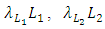 and
and 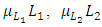 respectively. There is competition between the Cheetahs and the Lions.
2.1.2. The Model
The Model has four differential equations, for: Vegetation Biomass, Herbivores, Lions and Cheetahs.The first differential equation for Vegetation Biomass, it has two terms: the logistic growth equation: 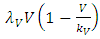 and the consumption term:
  According to the Logistic growth term of the ecosystem, can only support a maximum biomass
  .In the consumption term, there is an interaction between the Herbivores and the Vegetation biomass, with a negative sign of the coefficient of interaction
  because there is a decline of Vegetation biomass due to being fed on by the Herbivores. As the Vegetation Biomass increases, the consumption also increases, but there is a limit, the Herbivores won’t finish the whole volume of Vegetation. Thus, there is a limit of consumption. This means that even if there will be a lot of Vegetation Biomass. Due to that, a term
  of the Vegetation biomass at which it will be a half of the maximum rate of interaction introduced in the denominator of the term, thus mathematically;
  .The second differential equation is for the Herbivores. It has five terms: the reproduction term,
  the mortality term,
  the Vegetation Biomass consumption term,
  the rate at which the Herbivores are consumed by the Lions,
  and the rate at which the Herbivores are consumed by the Cheetahs,
  In the reproduction term, there is a birth rate of the herbivores due to natural per capita birth rate
  of the Herbivores population. In the mortality term, there is a death rate of herbivores that is negative due to the per capita mortality rate
  of the Herbivores population. The Vegetation Biomass consumption term represents the gained number of Herbivores born per volume of Vegetation consumed with a positive coefficient
  . The rate at which the Herbivores are consumed by the Lions is the fourth term,
  It has a negative interaction coefficient
  due to the decline of Herbivores’ population as the Lions prey on them. The rate at which the Herbivores are consumed by Cheetahs is the fifth term,
  It has a negative interaction coefficient
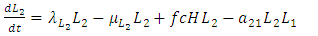
  due to the decline of Herbivores’ population as the Cheetahs prey on them. The third differential equation is for the Lions. It has four terms: the reproduction terms for Lions,
  the mortality term for Lions,
  the rate at which the herbivores are consumed by Lions,
  and the rate at which the Lions and Cheetahs compete,
  In the reproduction term for the Lions,
  there is a positive natural per capita birth rate of the Lions
  . In the mortality term for Lions,
  there is a positive per capita death rate of the Lions,
  . Then it is the rate at which the Herbivores are consumed by Lions, at a positive coefficient of interaction
  , thus increasing the Lions population by a multiple magnitude of
  . The rate at which the Lions compete with the Cheetahs has a negative coefficient of interaction
  The differential equation for the Cheetahs has four terms: the reproduction terms for Cheetahs,
  the mortality term for Cheetahs,
  the rate at which the Herbivores are consumed by the Cheetahs,
  and the rate at which the Lions compete with the Cheetahs,
  In the reproduction term for the Cheetahs, there is a birth rate coefficient of the Cheetahs
  that is positive due to its natural per capita birth rate of the Cheetahs population
  . In the mortality term for Cheetahs, there is a death rate coefficient of Cheetahs
  . Then it is the rate at which the Herbivores are consumed by the Cheetahs, with a positive coefficient of interaction
  as the product of the number of Cheetahs reproduced per Herbivores consumed, and thus increasing the Cheetahs population by a factor of
  . The rate at which the Cheetahs compete with the Lions has a negative coefficient of interaction
  .These are the Variables:
Table 1. The Variables
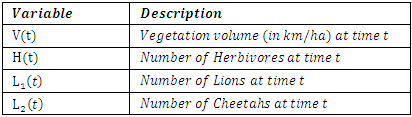 |
| |
|
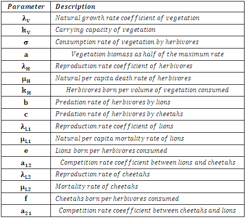
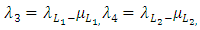
Also according to the above description, the following table has the Parameters.Table 2. The Parameters
 |
| |
|
The following is the model derived from the description of the dynamics of the ecosystem: 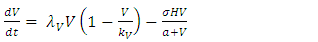 | (1) |
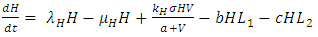 | (2) |
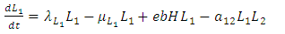 | (3) |
 | (4) |
2.1.3. Analysis of the Model
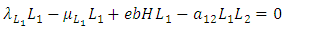
In order to establish the equilibrium points we set the derivatives in the model equal to zero. Thus, we have: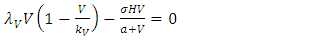 | (5) |
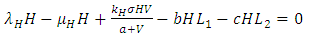 | (6) |
 | (7) |
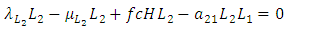 | (8) |
In this model, the equilibrium points of interest are the feasible points which satisfy: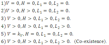 After using MAPLE, among the six, there are only two feasible solutions of the equilibrium points:
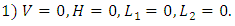 Interpretation:This is the point where there is extinction of all the species. That is there are no vegetation, no herbivores and no carnivores. This is unlikely to happen.
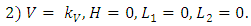 Interpretation:This is the point where only the vegetation exists at its own growth rate. No Herbivores to feed on it. It will grow logistically until it reaches it’s limit
  .Testing for local stability for that point, then, the eigenvalues are:
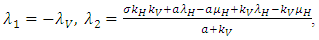
 Conclusion: For stability all the eigenvalues should be negative. Since only the first eigenvalue is negative and the rest are positive, hence the point is unstable.
2.1.4. Numerical Investigation of the Model
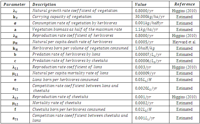
We initialize the parameter values to fit the Model and thus produce feasible plots. It should be noted that most of the parameter values are not available in the literature. Hence, we estimated them. The estimated parameters produced the best fit plots, for the years 2007-2019.These are:Table 3. The Initial Estimated Parameter Values
 |
| |
|
We then use the Least Mean Square Method to simulate the Model using the estimated parameter values and initial values of variables, and a time span of 13 years. With the assumption that there existed no real data at hand, we then created noisy data by adding Relative Gaussian Noisy to the simulated variable solution. The idea of corrupting the solution of ODEs is to treat a noisy data as a true data. We then estimate the parameters by minimizing the sum of squares of residuals.We compare the initial parameters used to simulate the model with the estimated parameter values.
3. Results and Discussion
The Results of the Estimated ParametersAfter simulation, we get the estimated parameter values which are all positive and are correlating with the initialized estimated parameters.Table 4. The Estimated Parameter Values
 |
| |
|
We also simulate the model, this time using the estimated parameter values and the real data, with the same time span and get the best fit plots. (Here, the green line represents the Heuristic data and the blue line represents the Model).The Results of the Population Dynamics for the years 2007-2019The results of the four best fit graphs summarize the Population Dynamics of the Vegetation biomass, Herbivores, Lions and Cheetahs populations respectively, when there is no Great Migration under normal conditions.For the Vegetation fitting curve in Figure 1, initially, the Vegetation biomass was 11,000kg/ha/yr in 2007, at a per capita growth rate of 0.8000/yr, with a carrying capacity of 30,000kg/ha with a coefficient of consumption of Vegetation biomass by Herbivores of 0.001km/haH yr, by initial estimations.After simulation, the results shows that the Vegetation volume increases approximately from 11,000kg/ha in 2007 to 11,344kg/ha/yr in 2008 and increases to 11684kg/ha/yr in 2009, at per capita growth rate of 0.8287/yr. The carrying capacity is approximately 35,234kg/ha.For the Herbivores fitting curve in Figure 2, initially, the population was 1,400,000 Herbivores in 2007. The per capita birth rate is 0.8000/yr, and the mortality rate of 0.0005/yr. The predation rate of Herbivores by Lions is 0.00007/L_1/yr, the predation rate of Herbivores by Cheetahs is 0.00006/L_2/yr, by initial estimations.The simulation results shows that the Herbivores Population increases from 1,400,000 Herbivores in 2007 to approximately 1,488,676 Herbivores Population size in 2008, increases to 1,579,995 Herbivores in 2009 then increases to 1,672,724 Herbivores in 2010, at per capita birth rate 0.8044/yr, and the mortality rate of approximately 0.00034/yr. The predation rate of Herbivores by Lions is approximately 0.0000812, the predation rate of Herbivores by Cheetahs is 0.0000512 approximately.For the Lions fitting curve in Figure 3, the results shows that the Lions Population was 700 in 2007, reproducing at the per capita birth rate of 0.003000/yr while dying at the mortality rate of 0.00009/yr. The competition rate between the Lions and Cheetahs is 0.0020/L_2/yr, by initial estimations.The simulation results show that the Lions’ Population increases from 700 in 2007 to approximately 933 Lions Population size in 2008, increases to 1,254 in 2009, to 2,286 in 2011, then continues to increase to 9,066 in 2019. They reproduce at per capita birth rate of 0.00205/yr while dying at the mortality rate of 0.000061/yr. The competition rate between the Lions and Cheetahs is 0.00101/L_2/yr.For the Cheetahs fitting curve in Figure 4, the results shows that the Cheetahs Population decreases from 60 in 2007 and onwards, reproducing at the per capita birth rate of 0.001/yr while dying at the mortality rate of 0.0002/yr. The competition rate between the Cheetahs and Lions is 0.001/L_1/yr, by initial estimations.The simulation results show that the Cheetahs’ Population decreases from 60 in 2007 to approximately 53 Cheetahs Population size in 2008, decreases to 17 in 2011 then drops to 1 in 2014, and goes to extinction. They reproduce at per capita birth rate of 0.000434/yr while dying at the mortality rate of 0.000286/yr. The competition rate between the Cheetahs and Lions is 0.001108/L_1/yr.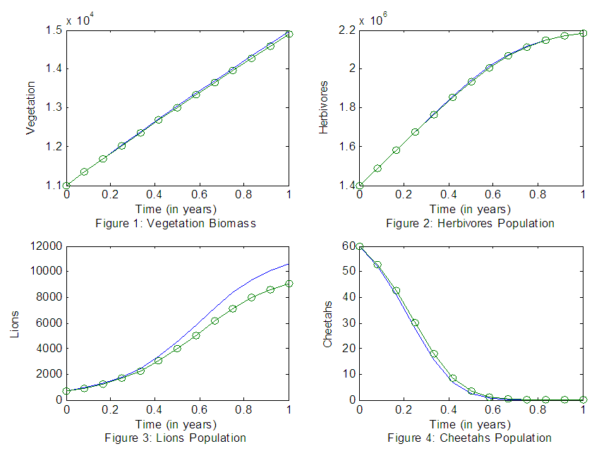 | Figures 1-4. The graphs of the best fitting curves of Vegetation, Herbivores, Lions and Cheetahs for the years 2007-2019 |
4. Conclusions
We conclude that, from the results of the best fitting graphs, first of all, the Vegetation volume increases. This is the food the Herbivores to feed on, so it affects the Herbivores population.Secondly, the Herbivores population increases. We suggest the increase is due to the availability of Vegetation for them to feed on.Thirdly, the Lions Population increases. We presume it is because of the existence of Herbivores Population abundantly as their prey due to the abundance of Vegetation volumes.Lastly, the Cheetahs Population, decreases. We suggest that the decrease is due to the competition between the Cheetahs against the increase of population of the Lions.
ACKNOWLEDGEMENTS
We would like to thank Dr. Isambi S. Mbalawata from AIMS in Tanzania for his technical support.
References
| [1] | Bedelian, C. (2014). Saving the Great Migrations: Declining Wildebeest in East Africa?. Environmental Development, 9, 101-109. |
| [2] | Caro, T., & Scholte, P. (2007). When protection falters. African Journal of Ecology, 45(3), 233-235. |
| [3] | Harris, G., Thirgood, S., Hopcraft, J. G. C., Cromsigt, J. P., & Berger, J. (2009). Global decline in aggregated migrations of large terrestrial mammals. Endangered Species Research, 7(1), 55-76. |
| [4] | Ngana, J. J., Luboobi, L. S., & Kuznetsov, D. (2014). Mathematical model for the population dynamics of the Serengeti ecosystem. Applied and Computational Mathematics, 3(4), 171-176. |
| [5] | Owen-Smith, N., & Ogutu, J. (2012). Changing rainfall and obstructed movements: impact on African ungulates. Wildlife conservation in a changing climate, 153. |
| [6] | Sinclair, A. R. E., Hopcraft, J. G. C., Olff, H., Mduma, S. A., Galvin, K. A., & Sharam, G. J. (2008). Historical and future changes to the Serengeti ecosystem. Serengeti III: human impacts on ecosystem dynamics, 7-46. |

 Abstract
 Reference
 Full-Text PDF
 Full-text HTML