Janeth J. Ngana 1, Livingstone S. Luboobi 2, Okelo J. Abonyo 3
1Pan African University, Institute for Basic Sciences, Technology and Innovation, Nairobi, Kenya
2Strathmore University, Nairobi, Kenya
3Jomo Kenyatta University of Agriculture and Technology, Nairobi, Kenya
Correspondence to: Janeth J. Ngana , Pan African University, Institute for Basic Sciences, Technology and Innovation, Nairobi, Kenya.
| Email: |  |
Copyright © 2019 The Author(s). Published by Scientific & Academic Publishing.
This work is licensed under the Creative Commons Attribution International License (CC BY).
http://creativecommons.org/licenses/by/4.0/

Abstract
Very few ecological studies have modeled Population Dynamics of the Serengeti Ecosystem under variable weather conditions. This paper seeks to analyze and forecast the trends of the Population Dynamics of the migratory ungulates of the Serengeti Ecosystem, under consistent monthly rainfalls and under varying rainfalls, when there is Climate Change. To get the Population Dynamics, we formulated a model of five Ordinary Differential Equations for: Vegetation biomass, Herbivores, Lions, Cheetahs and Crocodiles. For analysis of the model data, we used the Least Mean Square method. We found that in general, as the Vegetation volume grows logistically yearly, the Herbivores population decreases and as a result the populations of the Lions, the Cheetahs and the Crocodiles also decrease.
Keywords:
Cheetahs, Crocodiles, Herbivores, Lions, Maasai-Mara, Population Dynamics, Serengeti ecosystem, Vegetation biomass
Cite this paper: Janeth J. Ngana , Livingstone S. Luboobi , Okelo J. Abonyo , Mathematical Model for the Serengeti Ecosystem under Weather Variations, American Journal of Computational and Applied Mathematics , Vol. 9 No. 3, 2019, pp. 85-95. doi: 10.5923/j.ajcam.20190903.04.
1. Introduction
According to United Nations Fact sheets on Climate Change (UN Climate Change Conference Nairobi, 2006), Africa is the continent most vulnerable to the impacts of Climate Change. The continent is facing wide range of impacts including droughts and floods. In the near future, Climate Change will contribute to changes in natural ecosystems and loss of biodiversity.The Serengeti ecosystem supports an abundant community of herbivores and carnivores (Sinclair at al., 2003). Population of many wildlife species are declining, concurrent with changes in climate (Bartzke et al., 2018). Climate warming can change rainfall seasonality and cycle periods by modulating ocean-atmospheric circulation (Bartzke et al., 2018).A better understanding of rainfall dynamics is indispensable for developing biodiversity conservation measures likely to be effective under Climate Change (Maclean & Wilson, 2011). These changing rainfall patterns have implications for animal population dynamics.Rainfall is the principal driver of the Population dynamics of the savannah Herbivores (Ogutu & Owen-Smith, 2005; Ogutu et al., 2008), because it controls plant biomass production (Boutton, et al. 1988; Sankaran et al., 2005), and plant nutrient concentration (Boutton et al., 1988), which affect herbivores birth (Ogutu et al., 2008) and survival (Owen-Smith et al., 2005) rates , susceptibility to predation (Mills et al., 1995) and ultimately biomass (Coe, 1977; Fritz & Duncan, 1994). Not surprisingly, oscillatory dynamics in ungulate population size (Ogutu & Owen-Smith, 2005) and ungulate fecundity (Ogutu et al., 2014) are coupled with inter-annual and seasonal rainfall oscillations in African Savannah, respectively (Bartzke et al., 2018).During low rainfall years, animals are forced to travel longer distances between water and foraging grounds, making their offspring more vulnerable to predation (Loveridge et al., 2006).In addition to rainfall variability, water flow in Masai Mara River has been declining as a consequence of upstream deforestation of the Mau forest and excessive water abstraction for irrigation in Kenya (Gereta et al., 2009).Declining ungulates population within national parks and wildlife reserve have become an object of growing concern with regard to the preservation of Africa’s rich large mammals diversity (Caro & Scholte, 2007), especially in the case of migratory populations (Harris et al., 2009; Owen-Smith & Ogutu, 2012).Many studies have embarked on researches on the temperature and its dependence to functional responses as the impact of climate change. Very few have researched on rainfall-dependence to functional responses of several species.Ngana et al. (2014) did a research on the population dynamics and the Great Migration of the Serengeti ecosystem. They used a prey-predator model with migration to get the ODE’s for the Vegetation biomass, Herbivores, the Lions and Crocodiles. They did a simulation to get the population dynamics, without considering any impact of Climate Change. The result was that the Herbivores population was increasing, as well as the Carnivores population.In this paper, we consider the dynamics of the Serengeti Ecosystem under consistent rainfall including the impact of the Great Migration. We formulate a Food Chain Model consisting five Ordinary Differential Equations for the interaction between, Vegetation; Herbivores: Wildebeests, Zebra and Thompson’s Gazelles; and the Carnivores: the Lions, the Cheetahs and the Crocodiles. We analyze the model using the estimated initial values of the variables values. By simulation, we get estimated values of the parameters and then deduce the Population Dynamics of the five species. The Vegetation biomass is the food for the Herbivores. The Herbivores are preyed on by the Carnivores: the Lions, the Cheetahs and the Crocodiles.
1.1. Model Formulation
1.1.1. The Assumptions
The Assumptions for formulating the Model under Weather Variations.1. The Vegetation grows according to a logistic model with carrying capacity of  2. There is a constant consumption rate
  of Vegetation by a Herbivore.3. The ungulates will migrate due to extremes of low rainfall.4. The migratory animals are considered to the Wildebeest, Zebra and Thomson’s Gazelles.5. The predators are considered to be Lions, Cheetahs and Crocodiles.In modeling the ecological system, the Vegetation growth rate
  is assumed to have a logistically growing term in the absence of the Herbivores with an intrinsic growth rate
  and the carrying capacity
  The Herbivores, which are the Wildebeest, Zebra and Thompson’s Gazelles,
  reproduce at their average per capita rate of birth of
  They die naturally even in the presence of Vegetation, at their average per capita mortality rate
  They reduce at the rate of
  where b is the coefficient of interaction between the Herbivores and the Lions which results in a reduction of Herbivores population, when interacting with Lions. They reduce at the rate of
  where c is the coefficient of interaction between Herbivores and Cheetahs populations which results to a reduction of Herbivores population, when interacting with Cheetahs. They also reduce at the rate of
  where d is the coefficient of interaction between Herbivores and the Crocodiles populations which results to a reduction of Herbivores population, when interacting with the Crocodiles. For the Lions, Cheetahs and Crocodiles, the rates of change
  and
and  respectively, depend on their interactions with the Herbivores. The per capita reproduction rates and mortality rates are:
  and
and  respectively.
1.1.2. The Model
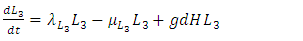
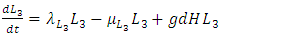
The Models has five differential equations, for: Vegetation Biomass, Herbivores, Lions, Cheetahs and Crocodiles.The first differential equation for Vegetation Biomass, it has two terms: the logistic growth equation:  with consistent rainfall
  and:
and:  with rainfall weather variation
  and the consumption term:
  where the Herbivores consume Vegetation biomass. According to the Logistic growth term, the ecosystem can only support a maximum Vegetation biomass
  In the consumption term, there is an interaction between the Herbivores and the Vegetation biomass, with a negative sign of the coefficient of interaction
  because there is a decline of Vegetation biomass due to being fed on by the Herbivores. As the Vegetation Biomass increases, the consumption also increases, but reaching a limit; for the Herbivores won’t finish the whole volume of Vegetation. Thus, there is a limit to consumption, even if there will be a lot of Vegetation Biomass. The consumption rate is modeled as:
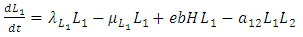
  in which a is the Vegetation biomass at which the consumption rate is half of the maximum rate.The differential equation for the Herbivores has eight terms: the reproduction term,
  the mortality term,
  the Vegetation Biomass consumption term,
  the rate at which the Herbivores are consumed by the Lions,
  the rate at which the Herbivores are consumed by the Cheetahs,
  the rate at which the Herbivores are consumed by the Crocodiles,
  the emigration and immigration terms with consistent rainfall
  and
and  respectively, and the emigration and immigration terms for varying rainfall
  are:
are:  and
and  , respectively. The terms have negative exponential functions due to opposite seasons between Serengeti ecosystem in Tanzania and Maasai-Mara ecosystem in Kenya. When it is a dry season for Serengeti, it is a wet season for Maasai-Mara, and so the Herbivores emigrate from Tanzania to Kenya, and vice versa; hence the Great Migration due to the Herbivores movement in search for food and water. In the reproduction term, there is a birth rate of the herbivores due to natural per capita birth rate
  of the Herbivores population. In the mortality term, there is a death rate of herbivores that is negative due to the per capita mortality rate
  of the Herbivores population.The Vegetation Biomass consumption term represents the gained number of Herbivores born per biomass of Vegetation consumed with a positive coefficient
  . The rate at which the Herbivores are consumed by the Lions is,
  while the Herbivores are consumed by Cheetahs at the rate
  . The rate at which the Herbivores are consumed by the Crocodiles is
  During the consistent rainfall
  the rate at which the Herbivores emigrate from Serengeti, Tanzania to Masai Mara, Kenya is,
  The rate at which the Herbivores immigrate to Serengeti, Tanzania from Masai-Mara, Kenya is
  During the varying rainfall
  the rate at which the Herbivores emigrate from Serengeti, Tanzania to Masai Mara, Kenya is the rate,
  The rate at which the Herbivores immigrate to Serengeti, Tanzania from Maasai-Mara, Kenya is
 (Thus, mathematically when there is no food in Tanzania;
  and no rain
  then the migratory animals emigrate from Tanzania to Kenya, because the emigration term
  When plenty of vegetation
  and wet season
 then the migratory animals immigrate from Kenya to Tanzania, because the immigration term is:
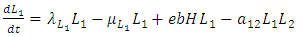
 The differential equation for the Lions has four terms: the reproduction terms for Lions,
  the mortality term for Lions,
  the rate at which Lions, benefit from the Herbivores that are consumed
  and the rate at which the Lions and Cheetahs compete,
  The per capita reproduction rate and the mortality rates of Lions are
  and
and  respectively.The Herbivores are consumed by Lions, at a positive coefficient of interaction b, and Lions are born per Herbivores consumed at a magnitude of e.The rate at which the Lions compete with the Cheetahs has a negative coefficient of interaction
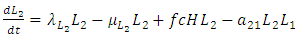
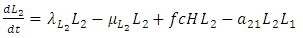
  due to its decreasing effect of the Lions population.The differential equation for the Cheetahs has four terms: the reproduction terms for Cheetahs,
  the mortality term for Cheetahs,
  the rate at which the Herbivores are consumed by the Cheetahs,
  and the rate at which the Lions compete with the Cheetahs,
  For the Cheetahs, the per capita birth and death rates are
  respectively.The rate at which the Herbivores are consumed by the Cheetahs, with a positive coefficient of interaction c as the product of the number of Cheetahs reproduced per Herbivores consumed, and thus increasing the Cheetahs population by a factor of f. The rate at which the Cheetahs compete with the Lions has a coefficient of interaction
  due to competition. The differential equation for the Crocodile has three terms: the reproduction terms for Crocodiles,
  the mortality term for Crocodiles,
  and the rate at which the Herbivores are consumed by the Crocodiles,
  In the reproduction term for the Crocodiles, there is a per capita birth rate coefficient of the Crocodiles
  In the mortality term for Crocodiles, there is a death rate coefficient of Crocodiles
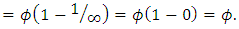
  Then it is the rate at which the Herbivores are consumed by the Crocodiles, with a positive coefficient of interaction d as the product of the number of Crocodiles reproduced per Herbivores consumed, and thus increasing the Crocodiles population by a factor of g.In summary the Variables are listed in Table 1.
Table 1. The Variables
 |
| |
|
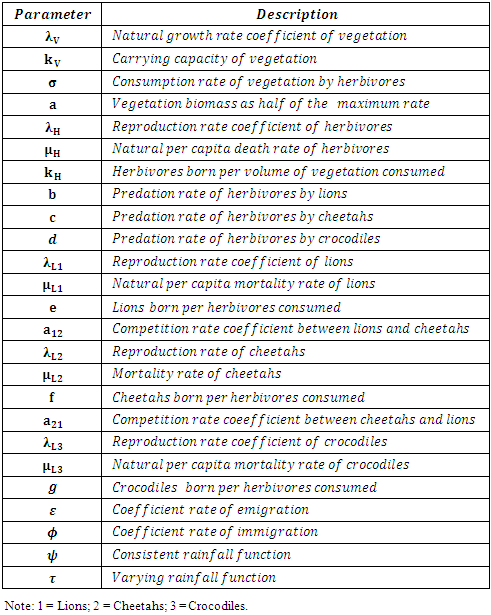
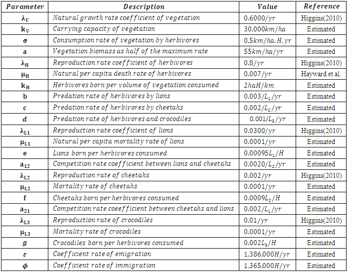
Also according to the above description, the parameters are listed in Table 2.Table 2. The Parameters
 |
| |
|
Based on the description of the dynamics of the Serengeti ecosystem, for consistent rainfall, we develop the model consisting of the differential equations (1) – (5).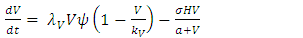 | (1) |
 | (2) |
 | (3) |
 | (4) |
 | (5) |
Also, based on the description of the dynamics of the Serengeti ecosystem, for varying rainfall, as described above, we modify the equations (!) – (5) to the model consisting of differential equations (6) – (10).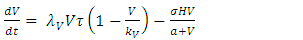 | (6) |
 | (7) |
 | (8) |
 | (9) |
 | (10) |
in which the initial values of the variables are non-negative.Under consistent rainfall  is constant, while for varying rainfall
  is becomes
  which depends on varying rainfall. Using the rainfall data available, we generate equations for
  and
and  rainfalls, and we use them to project the status of the Serengeti ecosystem.Using the Lagrange Interpolation formula, we get the equations for consistent rainfall,
  and varying rainfall,
  According to Lagrangian interpolation formula:
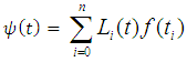 , where;
 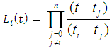 ; where,
  is the rainfall values as per month.From the available data, we express the consistent rainfall equation as follows:
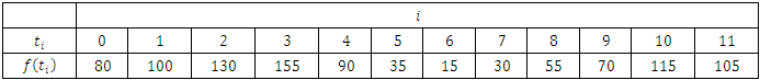 Then, at
  it implies,
 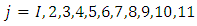 and
and  this implies;
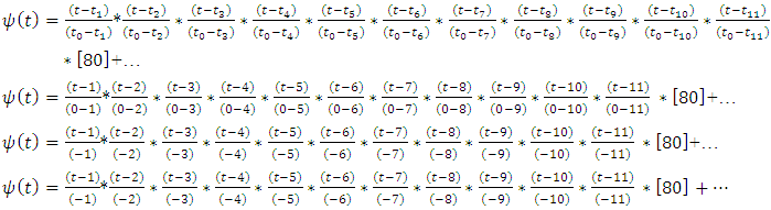 Thus;
Thus;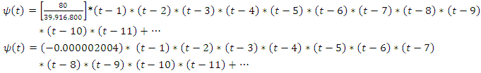 That is;
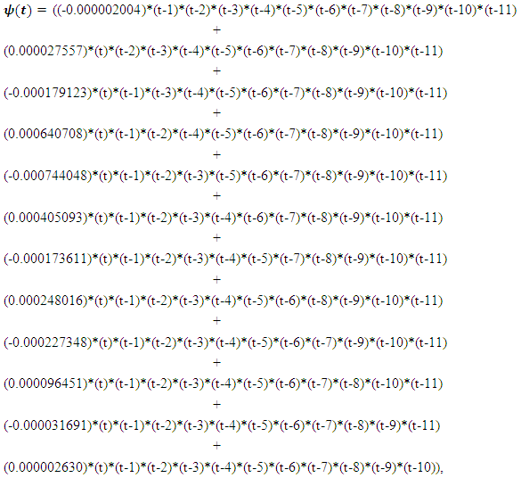 And, for varying rainfall data,
  becomes
  thus;
thus; 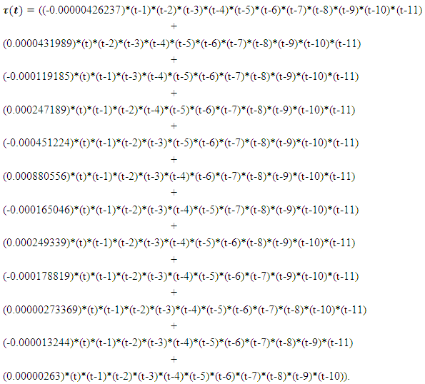 We then substitute the two into the two models, thus, the
  into the equations (1) and (2) and the
  into the equations (6) and (7) respectively and do simulation. (Here, the t is the time in months).
2. Rainfall Graphical Analysis
Graphs of consistent and varying rainfalls are analyzed. 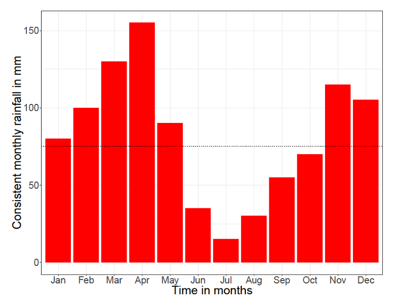 | Figure 1. The Annual Average consistent rainfall graph of Serengeti (Source: https://www.climatestotravel.com/climate/tanzania, Website Title: Tanzania climate: average weather, temperature, precipitation, best time) |
Figure 1 shows the monthly consistent rainfalls in general for Serengeti. The dotted line shows the annual average rainfall which is 82mm.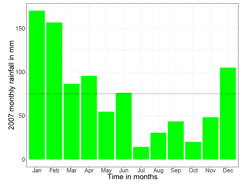 | Figure 2. The monthly rainfall graph for the year 2007 at Serengeti (Source: Tanzania Wildlife Research Institute (TAWIRI)) |
Figure 2 shows the monthly rainfalls for the year 2007. The dotted line shows the 2007 monthly average rainfall which is 75mm.Due to the scarcity of data from TAWIRI, 2007 is the only year with all the records from the stations of Serengeti. The other years have some records, but they are very scattered. 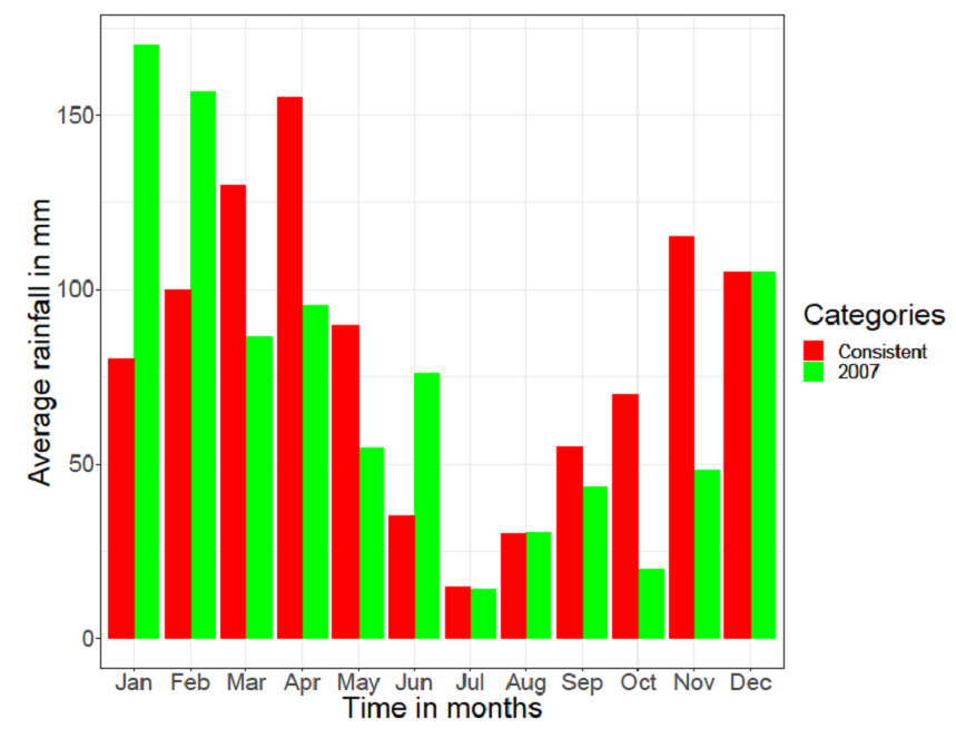 | Figure 3. The monthly rainfalls graphs for consistent and for the year 2007 at Serengeti (Source: Tanzania Wildlife Research Institute (TAWIRI)) |
Observation: From the annual average rainfalls of general consistent and varying rainfalls of 2007 respectively, it shows that there was a drop of 7mm on the annual average rainfall for the year 2007.
3. Numerical Investigation of the Model
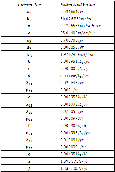
We initialize the parameters values to fit the Models and thus produce feasible plots. It should be noted that most of the parameter values are not available in the literature. Hence, we estimated them. The estimated values of the parameters that produced the best fit plots, from the month January to December, are as listed in Table 3.Table 3. The Initial Estimated Parameter Values for the Consistent and Varying Rainfalls
 |
| |
|
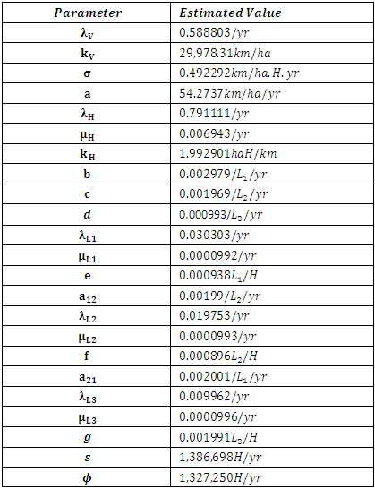
We then simulate the Model using the initial parameters’ values and initial values of the variables, and a time span of 12 months. With the assumption that there existed no real data at hand, we then created noisy data by adding Relative Gaussian Noisy to the simulated variable solution. The idea of corrupting the solution of ODEs is to treat a noisy data as a true data. We then estimate the Parameters by minimizing the sum of squares of residuals.By the Least Mean Square method and curve fitting, we simulate the model using the initial estimated parameters. The estimated parameters after simulations are all positive and are correlating with the initialized estimated parameters.Table 4. The Estimated Parameter Values for Consistent Rainfall
 |
| |
|
We now simulate the Model, using the parameter estimated values and the real data, over the same time span.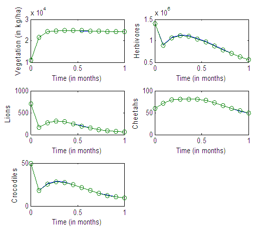 | Figure 4. The graphs of the best fitting curves of Vegetation biomass, Herbivores, Lions and Cheetahs from the months January to December under consistent rainfalls |
3.1. The Results of the Population Dynamics for the Annual Consistent Rainfall
The results of the five best fit graphs summarize the Population Dynamics of the Vegetation biomass, Herbivores, Lions, Cheetahs and Crocodiles populations respectively, when there is the Great Migration under consistent rainfall.For the Vegetation fitting curve, initially, the Vegetation biomass is 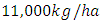 in January, at a per capita growth rate of
  with a carrying capacity of
 with a coefficient of consumption of Vegetation biomass by Herbivores of
  , by initial estimations.After simulation, the results shows that the Vegetation volume increases approximately from
  in January to
  in February and increases to
  in December, at growth rate of
  The carrying capacity is approximately
  For the Herbivores fitting curve, initially, the population is
  Herbivores in January. The per capita growth rate is
  and the mortality rate of
  The predation rate of Herbivores by Lions is
  the predation rate of Herbivores by Cheetahs is
  and where the predation rate of Herbivores by Crocodiles is approximately
  by initial estimations.The simulation results shows that the Herbivores Population drops from
  Herbivores in January to approximately
  Herbivores Population size in February, increases to
  Herbivores in March then decreases to
  Herbivores in December, at per capital birth rate
  , and the mortality rate of approximately
  . The predation rate of Herbivores by Lions is approximately
  , the predation rate of Herbivores by Cheetahs is
  and the predation rate of Herbivores by Crocodiles is approximately
  For the Lions fitting curve, the results shows that the Lions Population decreases from 700 in January, reproducing at the per capita rate of
  while dying at the mortality rate of
  The competition rate between the Lions and Cheetahs is
  by initial estimations.The simulation results show that the Lions’ Population decreases from 700 in January to approximately 168 Lions Population size in February, increases to 268 in March, to 291 in May, then drops to 59 in December. They reproduce at per capita rate of
  while dying at the mortality rate of
  . The competition rate between the Lions and Cheetahs is
  For the Cheetahs fitting curve, the results shows that the Cheetahs Population decreases from 60 in January and onwards, reproducing at the per capita rate of
  while dying at the mortality rate of
  . The competition rate between the Cheetahs and Lions is
  by initial estimations.The simulation results show that the Cheetahs’ Population increases from 60 in January to approximately 79 Lions Population size in March, increases to 81 in May then drops to 50 in December. They reproduce at per capita birth rate of
  while dying at the mortality rate of
  . The competition rate between the Cheetahs and Lions is
  For the Crocodile fitting curve, the results shows that the Crocodiles’ Population decreases from 50 in January and onwards, reproducing at the per capita birth rate of
  while dying at the mortality rate of
  by initial estimations.The simulation results show that the Crocodiles’ Population decreases from 50 in January to approximately 18 Crocodiles Population size in February, increases to 29 in April and drops to 10 Crocodiles in December. They reproduce at per capita birth rate of
  while dying at the mortality rate of
  The emigration and immigration rates are
  and
and  Herbivores per year, respectively.
3.2. The Results of the Estimated Parameters for Varying Rainfalls
The estimated parameters are all positive and are correlating with the initialized estimated parameters.Table 5. The Estimated Parameter Values for the year 2007
 |
| |
|
We now simulate the Model, using these parameter estimated values, with the same time span.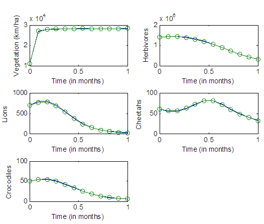 | Figure 5. The graphs of the best fitting curves of Vegetation biomass, Herbivores, Lions and Cheetahs from the months January to December for the year 2007 |
3.3. The Results of the Population Dynamics for the Year 2007
The results of the five best fit graphs summarize the Population Dynamics of the Vegetation, Herbivores, Lions, Cheetahs and Crocodiles respectively, when there is the Great Migration under varying rainfall.For the Vegetation fitting curve, initially, the Vegetation biomass is  in January, at a per capita growth rate of
  with a carrying capacity of
 with a coefficient of consumption of Vegetation biomass by Herbivores of
  by initial estimations.After simulation, the results shows that the Vegetation volume increases approximately from
  in January to
  in February and increases to
  in December, at growth rate of
  The carrying capacity is approximately
  For the Herbivores fitting curve, initially, the population is
  Herbivores in January. The per capita growth rate is
  and the mortality rate of
  The predation rate of Herbivores by Lions is
  the predation rate of Herbivores by Cheetahs is
  and where the predation rate of Herbivores by Crocodiles is approximately
  by initial estimations.The simulation results shows that the Herbivores Population increases from
  Herbivores in January to approximately
  Herbivores Population size in February, increases to
  Herbivores in March then decreases to
  Herbivores in December, at per capital birth rate
  and the mortality rate of approximately
  . The predation rate of Herbivores by Lions is approximately
  , the predation rate of Herbivores by Cheetahs is
  and the predation rate of Herbivores by Crocodiles is approximately
 For the Lions fitting curve, the results shows that the Lions Population decreases from 700 in January, reproducing at the per capita rate of
  while dying at the mortality rate of
  The competition rate between the Lions and Cheetahs is
  by initial estimations.The simulation results show that the Lions’ Population increases from 700 in January to approximately 769 Lions Population size in February, increases to 771 in March, drops to 530 in May, then drops to 25 in December. They reproduce at per capita rate of
  while dying at the mortality rate of
  . The competition rate between the Lions and Cheetahs is
  For the Cheetahs fitting curve, the results shows that the Cheetahs Population decreases from 60 in January and onwards, reproducing at the per capita rate of
  while dying at the mortality rate of
  . The competition rate between the Cheetahs and Lions is
  by initial estimations.The simulation results show that the Cheetahs’ Population decreases from 60 in January to approximately 56 Lions Population size in March, increases to 72 in May then drops to 32 in December. They reproduce at per capita birth rate of
  while dying at the mortality rate of
  . The competition rate between the Cheetahs and Lions is
  For the Crocodile fitting curve, the results shows that the Crocodiles’ Population decreases from 50 in January and onwards, reproducing at the per capita birth rate of
  while dying at the mortality rate of
  by initial estimations.The simulation results show that the Crocodiles’ Population increases from 50 in January to approximately 53 Crocodiles Population size in February, decreases to 49 in April and drops to 5 Crocodiles in December. They reproduce at per capita birth rate of
  while dying at the mortality rate of
  The emigration and immigration rates are
  and
and  Herbivores per year, respectively.
3.4. Discussion & Conclusions for the Constistent Rainfalls
From the results of the best fitting graphs, we conclude that, first of all, the Vegetation volume increases logistically. This is the food the Herbivores to feed on. It is suggestive that the growing trend is due to the nature of Vegetation biomass growth and due to the availability of rainfall consistently throughout the year.Secondly, the Herbivores population decreases. It is suggestive that the change is due to consumption of the Herbivores by the Lions, the Cheetahs and the Crocodiles.Thirdly, the Lions Population decreases. It is suggestive that it is because of the competition among them and the Cheetahs and Crocodiles in Herbivores consumption.Fourthly, the Cheetahs Population decreases. It is suggestive that the decrease is due to the competition among them and the Lions and Crocodiles in preying on Herbivores. Lastly, the Crocodiles Population decreases. It is suggestive that the drop is due to the competition among them, the Lions and Cheetahs in preying on Herbivores.
3.5. Conclusion & Discussion for Varying Rainfalls
From the results of simulation the model with the varying rainfalls’ best fitting graphs, we conclude that, first of all, the Vegetation volume increases. This is the food the Herbivores to feed on. It is suggestive that the growing trend is due to the nature of Vegetation biomass growth and due to the availability of rainfall though a bit varying throughout the year.Secondly, the Herbivores population decreases. It is suggestive that the change is due to consumption of the Herbivores by the Lions, the Cheetahs and the Crocodiles.Thirdly, the Lions Population decreases. It is suggestive that it is because of the competition among them and the Cheetahs and Crocodiles in Herbivores consumption.Fourthly, the Cheetahs Population decreases. It is suggestive that the decrease is due to the competition among them and the Lions and Crocodiles in preying on Herbivores. Lastly, the Crocodiles Population decreases. It is suggestive that the drop is due to the competition among them, the Lions and Cheetahs in preying on Herbivores.
4. General Conclusion
Generally, the Vegetation is growing logistically. It is suggestive that during the emigration of the Herbivores, the Vegetation biomass increases as the Herbivores are been killed by the Crocodiles and Carnivores as they emigrate, while the populations of Lions, Cheetahs and Crocodiles are declining. The reason could be due to competition.
ACKNOWLEDGEMENTS
The first author would like to thank Dr. Isambi S. Mbalawata from AIMS in Tanzania for his technical support.
References
| [1] | Caro, T., & Scholte, P. (2007). When protection falters. African Journal of Ecology, 45(3), 233-235. |
| [2] | Bartzke, G. S., Ogutu, J. O., Mukhopadhyay, S., Mtui, D., Dublin, H. T., & Piepho, H. P. (2018). Rainfall trends and variation in the Maasai Mara ecosystem and their implications for animal population and biodiversity dynamics. PloS one, 13(9), e0202814. |
| [3] | Boutton, T. W., Tieszen, L. L., & Imbamba, S. K. (1988). Biomass dynamics of grassland vegetation in Kenya. African Journal of Ecology, 26(2), 89-101. |
| [4] | Coe, M. J., Cumming, D. H., & Phillipson, J. (1976). Biomass and production of large African herbivores in relation to rainfall and primary production. Oecologia, 22(4), 341-354. |
| [5] | Fritz, H., & Duncan, P. (1994). On the carrying capacity for large ungulates of African savanna ecosystems. Proceedings of the Royal Society of London. Series B: Biological Sciences, 256(1345), 77-82. |
| [6] | Harris, G., Thirgood, S., Hopcraft, J. G. C., Cromsigt, J. P., & Berger, J. (2009). Global decline in aggregated migrations of large terrestrial mammals. Endangered Species Research, 7(1), 55-76. |
| [7] | Loveridge, A. J., Hunt, J. E., Murindagomo, F., & Macdonald, D. W. (2006). Influence of drought on predation of elephant (Loxodonta africana) calves by lions (Panthera leo) in an African wooded savannah. Journal of Zoology, 270(3), 523-530. |
| [8] | Mills, M. G. L., Biggs, H. C., & Whyte, I. J. (1995). The relationship between rainfall, lion predation and population trends in African herbivores. Wildlife Research, 22(1), 75-87. |
| [9] | Ngana, J. J., Luboobi, L. S., & Kuznetsov, D. (2014). Mathematical model for the population dynamics of the Serengeti ecosystem. Applied and Computational Mathematics, 3(4), 171-176. |
| [10] | Ogutu, J. O., & Owen-Smith, N. (2005). Oscillations in large mammal populations: are they related to predation or rainfall?. African Journal of Ecology, 43(4), 332-339. |
| [11] | Ogutu, J. O., Piepho, H. P., Dublin, H. T., Bhola, N., & Reid, R. S. (2008). Rainfall influences on ungulate population abundance in the Mara-Serengeti ecosystem. Journal of Animal Ecology, 77(4), 814-829. |
| [12] | Owen-Smith, N., Mason, D. R., & Ogutu, J. O. (2005). Correlates of survival rates for 10 African ungulate populations: density, rainfall and predation. Journal of Animal Ecology, 74(4), 774-788. |
| [13] | Owen-Smith, N., & Ogutu, J. (2012). Changing rainfall and obstructed movements: impact on African ungulates. Wildlife conservation in a changing climate, 153. |
| [14] | Sinclair, A. R. E., Mduma, S., & Brashares, J. S. (2003). Patterns of predation in a diverse predator–prey system. Nature, 425(6955), 288. |
| [15] | Washington, R., Harrison, M., Conway, D., Black, E., Challinor, A., Grimes, D., & Todd, M. (2006). African climate change: taking the shorter route. Bulletin of the American Meteorological Society, 87(10), 1355-1366. |
| [16] | Wolesensky, W. & Logan, J. D. (2007). An individual, stochastic model of growth incorporating state dependent risk and random foraging and climate. Mathematical Biosciences and Engineering, 4(1), 67-84. |

 Abstract
 Reference
 Full-Text PDF
 Full-text HTML