1. Introduction

Generating and assessing optimal design has remained prominent in the field of design of experiments (DOE) since the introduction of design optimality by [16]. Interestingly, optimal designs are of both theoretical and practical interests to experimenters since they are usually constructed to satisfy some specific practical purposes; such as getting precise parameter estimates or even with an aim of getting precise predictions. Although optimal designs may be obtained analytically, but analytic solutions are possible only in the simplest cases [8]. It is clear in literature that optimal design construction relies on certain principles or fundamental optimization techniques.

Most early algorithms involve iterative and exchange procedures. The iterative methods are based principally on the following;

i) Commence with a starting design, which is usually non-singular;

ii) Compute a sequence of designs iteratively, where the design is obtained by a small perturbation of the design

iii) Terminate the procedure by application of some stopping rule.

The use of exchange algorithms in optimal design construction basically involves the variance-exchange algorithms and coordinate-exchange algorithms. Early algorithms using exchange procedures include [2], [6], [8], [15], [19], [20], [29], etc. For instance, the Detmax algorithm of [19] is a point exchange algorithm that exchanges a point in a current design with a point from the candidate set while looking out for improvement in the selected optimality criterion. The coordinate-exchange algorithm of [18] exchanges every coordinate of a random starting design element by element for an optimal point until no further improvement in the optimality criterion is possible.

[26] introduced a combinatorial method in the problem of constructing D-optimal exact designs. The method is based on the combinatorics of the design points that make up the experimental region. The design points are grouped according to their distances from the center of the design region and an optimal tuple of the group of points is obtained such that the design point in the optimal tuple maximixes the determinant of information matrix. Modifications of the combinatiorial method have been provided for varying experimental conditions as in [14] and for reduction in computational requirements as in [13]. The combinatorial method converges rapidly and absolutely to the desired N-point D-optimal design and is effective for determining optimal designs in block experiments as well as in non-block experiments for finite or infinite number of design points in the experimental region.

[11] employed the principles of the loss function for the purpose of constructing designs for non-standard second-order models. In specific terms, the first compound of the hat matrix associated with central composite designs was used to obtain modified central composite designs for non-standard second-order models. It was observed that for a full parameter second-order model, the diagonal elements of the hat matrix exhibited a unique property, where the diagonal elements associated with design points in a particular CCD portion are a constant for all design points in that portion. Specifically, vertex points have constant diagonal element say, 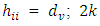axial points have constant diagonal element say, and center points have constant diagonal element say, However for a “non-standard” model, the associated hat matrix loses the unique property of its diagonal elements for an employed central composite design. [27] presented an algorithm for generating near G-optimal designs for second-order response surface models over cuboidal experimental region. The algorithm utilizes Brent’s minimization procedure with coordinate exchange to create second-order designs for two to five factors. Comparatively, the created designs are highly G-efficient having higher prediction variances over a vast majority of the design region.

Many computer-generated designs are created using popularly encountered alphabetic optimality criteria such as D-, G- and I-optimality criteria. The criterion of D-optimality seeks to obtain precise estimates of the model parameters. The criterion of G-optimality seeks to obtain good model prediction. I-optimality designs are useful in minimizing the average prediction variance over the design region. As in [27], computer-generated designs are not necessarily globally optimal designs but they are highly efficient for the specific criterion of interest. Moreover, for a pre-specified design size, there could be varying designs some of which have “inferior” calculated optimal measures.

Three level designs are often used for second-order response surface analysis and often require selecting design points that are without a large loss in efficiency. In all cases associated with discrete design runs , the selected design points are some points of the general factorial design associated with design variables. Some three-level second-order response surface designs often encountered in the literature for standard second-order models include Central Composite Designs, Box-Behnken Designs, Small Composite Designs, Hoke Designs, D-optimal Design, etc. For non-standard second-order models, computer-generated designs may be employed. These designs are implemented in some statistical software, including the Design-Expert and JMP. In this paper, diagonal elements of the hat matrix are employed in the selection of discrete design runs useful for constructing composite second-order designs for second-order models whether of standard or non-standard forms. The Hat-Matrix aided composite designs are comparable with Standard Response Surface Methodology (RSM) designs and Computer-Generated designs in their optimality and efficiency properties. The construction of the new designs depends on the principles of the loss function of [1], which are represented by the diagonal elements of the “Hat” matrix. Through the Hat-matrix, design points that enhance efficiency of second-order designs are selected. Unlike computer-generated designs which may not be unique for a specific model and which may present some less efficient designs, the Hat-Matrix (H-M) aided designs are unique and require at least two categories of discrete design runs formed from the complete factorial design runs only on the basis of the diagonal elements of the hat matrix that promote maximizing determinant of the information matrix thereby minimizing the loss function.

2. Some Second-Order Designs

Second-order designs are constructed to fit the Second-order model

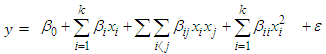(1)

Where the represent the model parameters whose estimates are obtained using the method of least squares.

As conventionally used, the estimated response, in matrix form, is

where the least squares estimate of vector of the unknown parameters is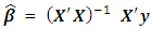

The unknown parameters are estimated on the basis of uncorrelated observations.

denotes the vector of observations and denotes the model matrix. From the least squares estimates of the unknown parameters, the estimated response is

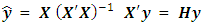(2)

where is called the hat matrix and puts the “hat” on the vector of fitted or estimated value.

2.1. 3-level Factorial Design

The factorial designs, whose history dates back to the 19^th century, are widely used in experimental situations and seen as more efficient than studying one factor at a time. The three-level series of factorial designs involving k factors each at three levels are extensions of the two-level series of factorial designs which involves k factors each at two levels. They are useful when there is suspected curvature in the response surface and the experimenter needs to evaluate the curvature. The three levels of a factorial design may be referred to as Low, Intermediate and High. The levels may be digitally represented as 0 (Low), 1 (Intermediate) and 2 (High). Specifically, a three-level factorial design has a center point included for each independent variable along with the high and low points. Inclusion of the third factor greatly increases the number of experiments. For a complete replicate of the factorial design, there are treatment combinations. As increases, the design requires many too many runs that may not be economical in practice. This results in confounding some effects in blocks and in the use of fractional factorial designs. Three-level factorial design is suitable for fitting second-order models when a first-order model suffers lack of fit due to interaction between variables and/or due to surface curvature.

2.2. Central Composite Design (CCD)

[5] developed central composite design. Over the years, it is the most popularly used design for RSM. The CCD is a very efficient design for fitting the second-order model in cuboidal or spherical region. Basically, a central composite design consists of a factorial portion (or a 2^k-p fractional factorial portion of resolution at least V), a set of 2k axial or star points of distances α from the origin and n_c center points. The values of the distance α and the number of center point n₀ are two important parameters in the design that must be specified. CCDs can be developed through a sequential experimentation by starting with factorial points, and then adding center and axial points. Adding the axial points will allow quadratic terms to be included into the model. The center runs contain information about the curvature of the surface. If curvature is significant, the additional axial points allow for efficient estimation of the quadratic terms. CCDs defined by some α values are rotatable and robust, although the total number of the design points of CCD could be extremely large, especially for large k as cited in [21].

2.3. Box-Behnken Designs

[3] and [4] developed efficient spherical three-level designs appropriate for fitting second-order (quadratic) response models. The designs are constructed by combining two-level (full or fractional) factorials with Balanced Incomplete Block Designs or Partially Balanced Incomplete Block Designs. In each block, a certain number of factors are put through all combinations for the factorial design, while the other factors are kept at the central values. Hence the designs do not contain any points at the vertices or face-center of the design region but rather at the center of the edges of the experimental space, thus avoiding extreme values for factor level combinations which may be impossible to test due to cost or physical process constraints [22]. The designs are rotatable or near-rotatable and require fewer experimental runs than the factorial technique. As the number of factor, increases, so does the run size of the designs. Additionally, the designs uses center runs to avoid singularity in the design matrix and to maintain favorable design qualities like good prediction variance [23]. Over the years, the designs have been improved in terms of rotatability, average prediction variance, D- and G-efficiency as in [17], [25], [31].

2.4. Small Composite Designs

[9] proposed small composite design which uses the idea of central composite design but the factorial portion is neither a complete factorial nor a resolution V fractional factorial design. The design is formed by replacing the factorial portion with a special resolution III fraction with no four-letter word as a defining relation. The fraction is such that two-factor interactions are not aliased with other two-factor interactions, thus resulting in a reduced number of design runs. Unfortunately, factorial portion linear main effect terms may be aliased with two-factor interaction terms thus resulting in poor estimation and prediction performance even though the design still allows for the estimation of all coefficients of the second-order model. [30] suggested replacing the factorial portion with an irregular fraction. [7] proposed the use of columns of Plackett-Burman designs.

2.5. Hoke Designs

Hoke [10] developed a class of second-order economical designs for 3 to 6 factors at 3 levels based on saturated and near-saturated irregular fractions of the factorial. Hoke designs are suitable for a cuboidal region of interest because it consist of a mixture of factorial, axial and edge points that create efficient second-order arrays for 3 to 6 factors. For each number of factors, several classes of the Hoke designs exist, and are denoted . [23] observed that symmetry of the designs across all factor is a good characteristic of all the versions of the design. The design classes and perform well with small variances for model parameters and prediction of new observations among the Hoke design choices.

2.6. Hybrid Designs

[28] developed a set of highly efficient saturated or near-saturated second-order designs. The construction of design involves the use of a central design for k-1 variables and the kth variable are determined in a way that allows the creation of symmetries in the design. This results in a class of designs that are economical, rotatable or near-rotatable.

2.7. Computer-Generated Designs

Computer-generated designs are non-standard response surface designs. The designs are appropriate when; (i) the experimental region is irregular; (ii) obtaining an efficient design for fitting a non-standard model and (iii) it is necessary to reduce the number of runs required by a standard response surface design. The computer-generated designs are constructed based on robustness (design insensitivity to specific set of assumptions and/or models) and most often uses alphabetic optimality criteria such as D-optimality and I-optimality. Optimal designs, satisfying specific optimality criteria, may be generated through the use of computer algorithms where all possible sets of candidate points are evaluated on the basis of empirical model of the response, available sample size, design factor values and certain other constraints [23], [24]. Computer-generated “optimal” designs can be created for any specified model, although caution should be taken when dealing with computer-generated designs as some generated designs may not be the “optimal” design within a class of designs.

2.8. Modified Central Composite Design

Modified central composite designs due to [12] are second-order designs for non-standard models constructed using principles of the loss function or equivalently first compound of matrix associated with hat matrix . They are formed by classifying the losses due to missing design points in the CCD portions. Where there are multiple losses associated with specified CCD portions, the design points having less impact may be deleted from the full CCD. This allows a possible increase in design efficiency and offers alternative designs, similar in the structure of CCDs, for non-standard models. In comparison with the central composite designs, the modified central composite designs have fewer design points and hence more economical for second-order non-standard models.

3. Methodology of Design Construction for the Hat-Matrix Aided Designs

For full unreplicated design runs, taking on the discrete variables levels -1, 0 and 1, we form a measure supported by the vector of design runs

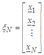where

is the discrete points in the geometric region

For 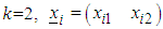; is a two component vector of dimension .

For 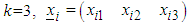; is a three component vector of dimension , and so on.

Associated with the design measure , for a full second-order model is the extended design matrix

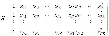For a non-standard model, where some parameters of the full p-parameter second-order model are not in the model, the columns of matrix are reduced to only the number of parameters in the non-standard model.

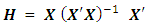
The hat matrix 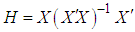which is a square symmetric idempotent matrix, is formed as a function of the extended design matrix X. The elements of the hat matrix have their values between 0 and 1. The diagonal elements, , of the hat matrix are such that

where p is the number of regression parameters including the intercept term.

is a measure of the distance between the x values for the case and the means of the x values for all cases.

The elements of the hat matrix H are denoted by

That is,

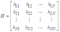The large value of indicates that the case is distant from the center for all cases. Aside giving a measure of the distance of the design point from the center of all design points, the hat matrix may also be used to quantify the effect of removing one or more observations from a complete data set. This idea is well explained in loss function approach of [1].

The use of loss function in studying the reduction in determinant of information matrix due to missing observations has effectively produced designs that are robust to missing observations. It is on the idea of loss function that the H-M aided design is based. The loss due to the design point is measured by the corresponding diagonal element of the hat matrix which in essence is the first compound of the hat matrix itself. The smaller a diagonal element of the hat matrix, the less the loss due to missing the associated design point. Correspondingly, the larger a diagonal element of the hat matrix, the more the loss due to missing the associated design point. In context of the loss function, we could eliminate some design points of the full factorial design associated with small loses. For the purpose of maintaining non-singular designs with reasonably few design points, design points in at least two compositions, contributing maximally to determinant of information matrix, on the basis of the diagonal element of the hat matrix, shall be included in the design. A common feature of such design points is that they have maximum diagonal elements or they constitute the best two categories of the diagonal elements.

4. Illustrations and Results

4.1. H-M Aided Composite Designs for Three-Variable Standard Seconds-Order Model

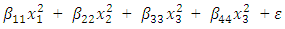
Consider the three-variable standard seconds-order model

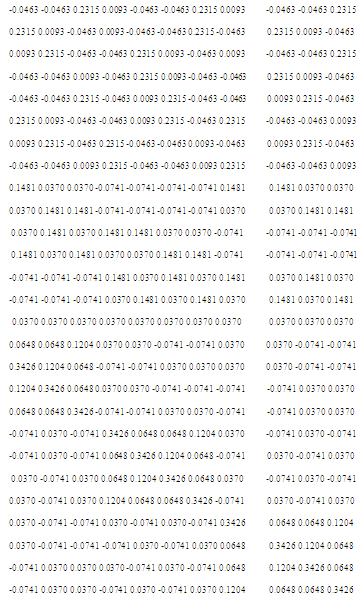
The hat matrix associated with discrete design runs (-1, -1, -1), (1, -1, -1), (-1, 1, -1), (1, 1, -1), (-1, -1, 1), (1, -1, 1), (-1, 1, 1), (1, 1, 1), (1, 0, 0), (-1, 0,0), (0, 1, 0), (0, -1, 0), (0, 0, 1), (0, 0, -1), (0, 0, 0), (1, 1, 0), (1, -1, 0), (-1, 1, 0), (-1, -1, 0), (0, 1, 1), (0, 1, -1), (0, -1, 1), (0, -1, -1), (1, 0, 1), (1, 0, -1), (-1, 0, 1), (-1, 0, -1) is as follows;

H =

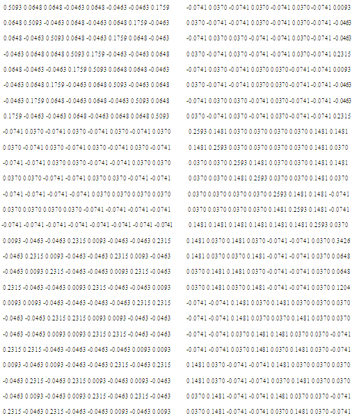
Design runs associated with the diagonal element 0.5093 and 0.3426 are used in the construction and yield the 20-point H-M aided design

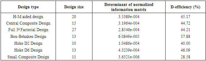
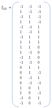D-efficiency of the 20-point H-M aided design has been compared with D-efficiencies of commonly encountered second-order designs and are tabulated in Table 1.

Table 1. D-efficiency values for some three-variable second-order designs

4.2. H-M Aided Composite Designs for Four-Variable Standard Seconds-Order Model

Consider the four-variable prior standard second-order model having model parameters

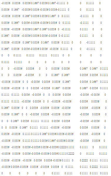
The hat matrix associated with discrete design runs is as in Appendix A. Design runs having the diagonal elements 0.2778 and 0.1944 are used in the construction and yield the 48-point H-M aided design

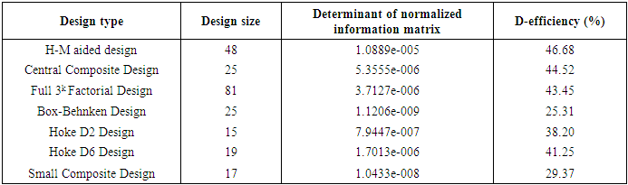
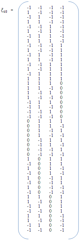D-efficiency of the 48-point H-M aided design has been compared with D-efficiencies of commonly encountered second-order designs and are tabulated in Table 2.

Table 2. D-efficiency values for some four-variable second-order designs

4.3. H-M Aided Composite Designs for Three-Variable Non-standard Seconds-Order Model in Five Parameters

Consider the three-variable non-standard second-order model having model parameters

The hat matrix associated with discrete design runs is as follows

H =

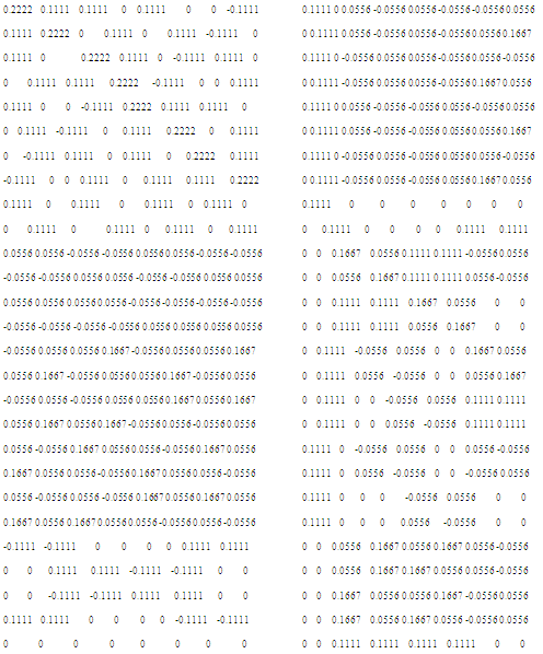
Two categories of design runs, each associated with the diagonal element 0.2222, are used in the construction and yield the 12-point H-M aided design

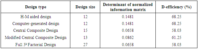
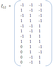D-efficiency of the 12-point H-M aided design has been compared with D-efficiencies of commonly encountered second-order designs and are tabulated in Table 3.

Table 3. D-efficiency values for some three-variable second-order designs on the non-standard model

4.4. H-M Aided Composite Designs for Three-Variable Non-standard Seconds-Order Model in Six Parameters

Consider the three-variable non-standard second-order model having model parameters

The hat matrix associated with discrete design runs is as follows

H =

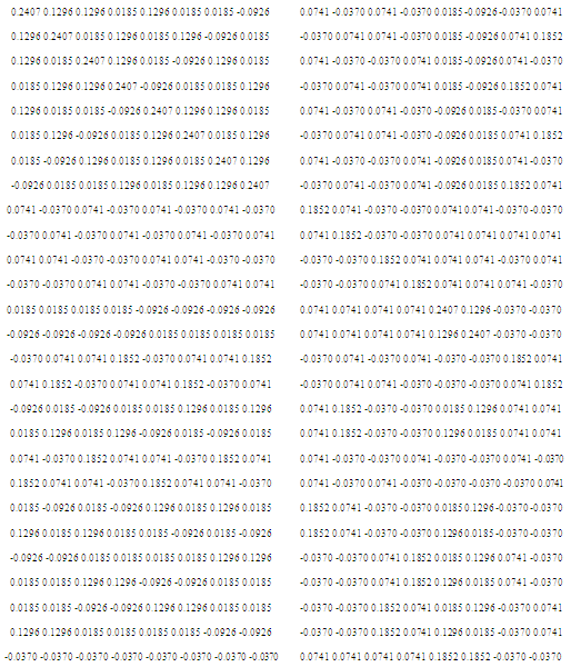
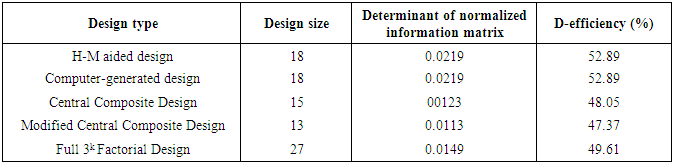
Three categories of design runs, each associated with the diagonal element 0.2407, are used in the construction and yield the 18-point H-M aided design

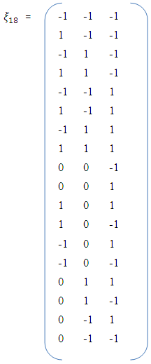D-efficiency of the 18-point H-M aided design has been compared with D-efficiencies of commonly encountered second-order designs and are tabulated in Table 4.

Table 4. D-efficiency values for some three-variable second-order designs on the non-standard model

4.5. H-M Aided Composite Designs for Four-variable Non-standard Seconds-Order Model in Nine Parameters

Consider the four-variable non-standard second-order model having model parameters

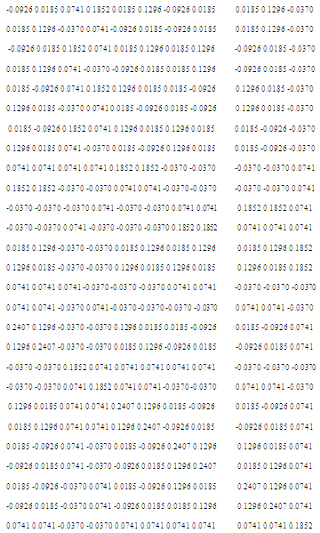
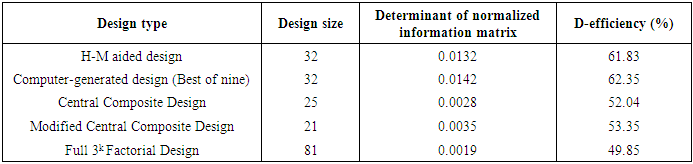
The hat matrix associated with discrete design runs is as in Appendix B. Two categories of design runs, with the diagonal elements 0.1543 and 0.1265, are used in the construction and yield the 32-point H-M aided design

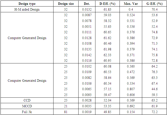
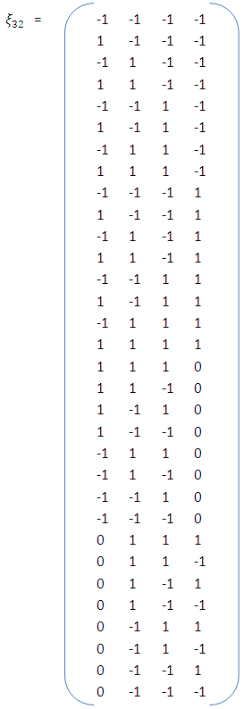D-efficiency of the 32-point H-M aided design has been compared with D-efficiencies of commonly encountered second-order designs and are tabulated in Table 5.

Table 5. D-efficiency values for some three-variable second-order designs on the non-standard model

Other measures derived from the information matrix associated with the four-variable designs for the nine-parameter non-standard model are as in Table 6. Multiple Computer-generated designs are obtained for user-specified design size. Unfortunately, some of the designs are not as efficient as the hat matrix aided design.

Table 6. Some Optimality measures for the four-variable designs associated with the nine-parameter non-standard model

5. Conclusions

Hat matrix has been employed as a viable tool for constructing seconds-order optimal designs that are comparable with commonly encountered designs for the second-order models. The Hat-Matrix aided composite designs depend on the principles of the loss function of [1], represented by the diagonal elements of the first compounds of the hat matrix. Unlike computer-generated designs which may not be unique for a specific model and for user-specified design size, the Hat-Matrix (H-M) aided designs are unique. The H-M aided designs are efficient and generally as good as the best computer-generated designs. Unfortunately, in event of multiple designs, most of the computer-generated designs are not as efficient as the hat-matrix aided design. H-M aided designs require at least two categories of discrete design runs formed from the complete factorial design runs only on the basis of the diagonal elements of the hat matrix that promote maximizing determinant of the information matrix thereby minimizing the loss function. A common feature of design points associated with H-M aided designs is that they have maximum diagonal elements or they constitute the best two categories of the diagonal elements.

Appendix A: Hat Matrix for Standard Second-Order Model in Four Design Variables and the Ordered Design Runs

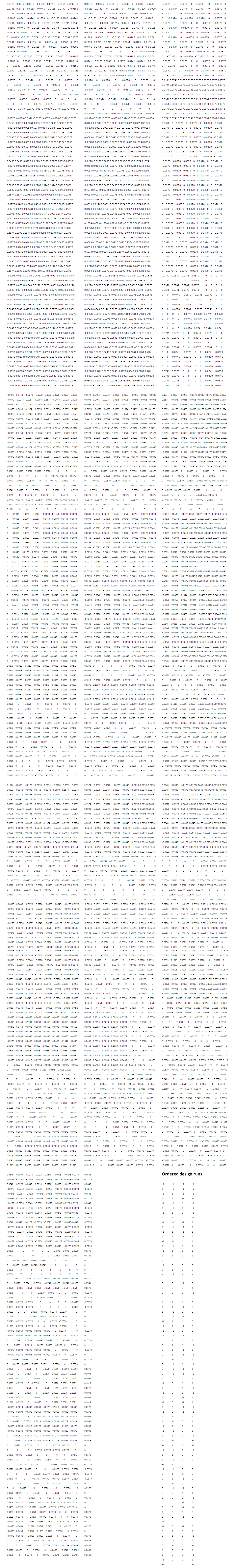Appendix A

Appendix B: Hat Matrix for Nonstandard Model four Design Variables and the Ordered Design Runs

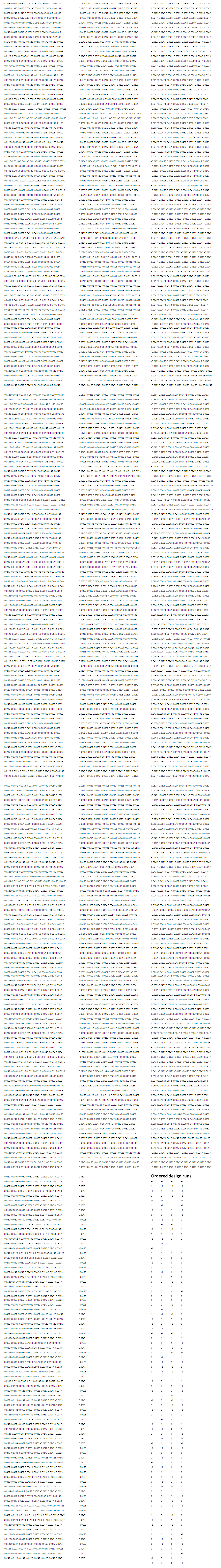Appendix B