Everestus Obinwanne Eze, Toochukwu Ogbonnia Oko, Chinenye Okorafor Goodluck
Department of Mathematics, Michael Okpara University of Agriculture Umudike, Abia State, Nigeria
Correspondence to: Everestus Obinwanne Eze, Department of Mathematics, Michael Okpara University of Agriculture Umudike, Abia State, Nigeria.
| Email: |  |
Copyright © 2019 The Author(s). Published by Scientific & Academic Publishing.
This work is licensed under the Creative Commons Attribution International License (CC BY).
http://creativecommons.org/licenses/by/4.0/

Abstract
In this paper, an approximate solution of the Sitnikov problem is investigated using both the Euler and fourth-order Runge-Kutta methods. The various values of eccentricities were obtained and demonstrated by simulations using MATCAD which showed that the range for the search of eccentricities can be narrowed down at different values of eccentricities, different sinusoidal frequencies were obtained.
Keywords:
Symmetric Periodic Solution, Sitnikov Problem, Fourth-order Runge-Kutta method
Cite this paper: Everestus Obinwanne Eze, Toochukwu Ogbonnia Oko, Chinenye Okorafor Goodluck, On the Approximation of Symmetric Periodic Solutions of the Sitnikov Problem, American Journal of Computational and Applied Mathematics , Vol. 9 No. 1, 2019, pp. 12-20. doi: 10.5923/j.ajcam.20190901.03.
1. Introduction
The Sitnikov problem describes the motion of a particle of negligible mass attracted by two equal masses 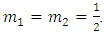 The primaries
  move on the plane
  , following an elliptic motion with eccentricity
  , while the massless body
  performs motion along an axis perpendicular to the primary orbit plane through the barycentre of the primaries. The minimal period of the elliptic motion is
  if the gravitational constant is assumed to be
  If
If  denotes the position of the particle
  in a coordinate system with origin at the centre of mass of the primaries, then the equation of motion of the Sitnikov problem becomes
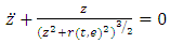 | (1.1) |
where  is the distance from the center of the orbit to
 is acceleration,
  is eccentricity and
  is the distance of the primaries to their center of mass and it is given by
 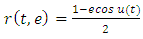 | (1.2) |
which is a circular or an elliptic solution of the Kepler problem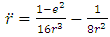 | (1.3) |
with eccentricity  respectively. Here
  is the eccentricity anomaly which is a function of time through Kepler equation
 | (1.4) |
without loss of generality, when  we take the origin of time in such a way that at
  the primaries are at the pericenter of the ellipse. We note that system (1.1) depends on one parameter, the eccentricity
  when the eccentricity
  is zero (that is, the primaries move on the circular orbit
  of the Kepler problem (1.3)), (1.1) becomes the equation of motion
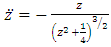 | (1.5) |
for the circular Sitnikov problem.More information can be found in [5] and in the more recent [1]. The existence of symmetric (even or odd) periodic solutions has been discussed in [2-4-6-7]. In [2] methods of local analysis were employed, and they got results which are valid only for small eccentricity  The papers [4, 6] considered arbitrary eccentricity from a theoretical perspective by using the global continuation method due to Leray and Schauder, and [6] found families of symmetric periodic solutions bifurcating from the equilibrium at the center of mass. These families were labelled according to the number of zeros in the same fashion as it occurs in the work by Rabinowitz [9] for other non-linearities. [7] combines Shooting arguments with Sturm comparison theory to prove the existence of odd periodic solutions with a prescribed number of zeros. While [3] presents a very complete description of the set of symmetric periodic solutions based on numerical computations. [8] discussed on the circular Sitnikov problem as a subsystem of the three-dimensional circular restricted three-body problem, where they used elliptic functions to give the analytical expressions for the solutions of the circular Sitnikov problem and for the period function of its family of periodic orbits. They also analyzed the qualitative and quantitative behaviour of the period function. The purpose of this note is to show that it is also possible to obtain numerical results for all values of the eccentricity using only very elementary tool, the fourth-order Runge-Kutta method. This paper is divided into sections. Section 2 is the definition and theorems which was used in the result while section 3 is the derivation of the fourth-order Runge-Kutta method, section 4 is the result obtained with numerical simulations and section 5 is conclusion.
2. Preliminary
Theorem 1. Precision of the Runge-Kutta methodsAssume that  is the solution of the problem
 | (2.1) |
If 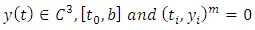 is the sequence of approximations generated by the Runge-Kutta method of order 2, then
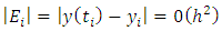
 Given the interval
  we satisfy that
 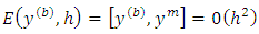 Theorem 2. Assume the existence of such a solution
  is guaranteed and unique, provided
  (i) is continuous in the infinite strip
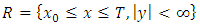 (ii) is more specifically Lipchitz continuous in the dependent variable
  over the same region
  that is there exist a positive constant
  such that for all
 Theorem 3. Suppose that
  is a nonempty, closed and bounded limit set of a planar flow, then one of the following holds:Ÿ
  is an equilibrium pointŸ
  is a periodic solutionŸ
  consists of a set of equilibria and connecting orbits between these equilibria.ProofWe consider
  for some
  The argument in the case of an
  set is similar.Let
  If
If  is not an equilibrium point, then
  must be a periodic solution and if
  is a periodic solution then
  and thus
  is also a periodic solution.Now we assume that
  is an equilibrium point. Then
  must consist entirely of equilibria since if there is a point
  that is not an equilibrium, then we know that
  is a periodic solution (and in particular contains no equilibrium). We note that since
  it follows that
  , where
  denotes the time-t flow. Hence
  and for the same reasons as before
  must be an equilibrium, since otherwise
  must be a periodic solution. Hence, we find that either
  is an equilibrium point, or that
  lies in the intersection between the stable and unstable manifolds of the equilibria
  (that is on a connecting orbit between equilibria).Theorem 4. For each integer
  there exists a unique solution
  of (1.1) satisfying the conditions,
  | (2.2) |
 | (2.3) |
The variational equation at the center of mass  will play an important role; it is the equation of Hill’s type
 | (2.4) |
Theorem 3. Assume that  are given integers. Then the following statements are equivalent:i) there exist a solution of (1.1) satisfying the condition in (2.2) and having exactly
  zero in the interval
  ii) the solution
  of (2.4) with initial conditions
  has more than
  zero in
3. Derivation of Fourth-order Runge-Kutta Method
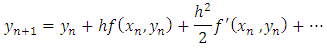
The simple Euler method comes from using just one term from the Taylor series for  expanded about
  . The modified Euler method can also be derived from using terms
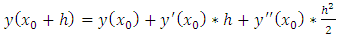 | (3.1) |
If we replace the second derivative with a backward-difference approximation,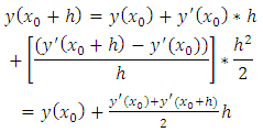 | (3.2) |
We get the formula for the modified method. What if we use more terms of the Taylor series? Two German mathematicians, Runge and Kutta, developed algorithms from using more than two terms of the series. We will consider only fourth-order formula. The modified Euler method is a second-order Runge-Kutta method.Second-order Runge-Kutta methods are obtained by using a weighted average of two increments to 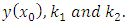 For the equation
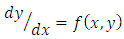
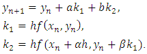 | (3.3) |
We can think of the values  as estimates of the change in
  when
when  advances by
  because they are the product of the change in
  and a value for the slope of the curve,
  The Runge-Kutta methods always use the simple Euler estimate as the first of
  the other estimate is taken with
  stepped up by the fractions
 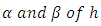 and of the earlier estimate of
  Our problem is to devise a scheme of choosing the four parameters,
  We do also by making equation (3.3) agree as well as possible with the Taylor-series expansion, in which the
 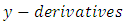 are written in terms of
  from
from 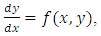
 An equivalent form, because
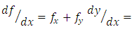
 is
is 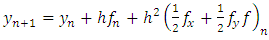 | (3.4) |
[All the derivatives in equation (3.4) are calculated at the point  .] we now rewrite equation (3.4) by substituting the definitions of
 | (3.5) |
To make the last term of equation (3.5) comparable to equation (3.4), we expand  in a Taylor series in terms of
  remembering that
  is a function of two variables, retaining only first derivative terms:
 | (3.6) |
On the right side of both equations (3.4) and (3.6),  and its partial derivatives are all to be evaluated at
  Substituting from equation (3.6) into equation (3.5), we have
 | (3.7) |
Equation (3.7) will be identical to equation (3.4) if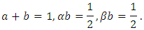 Note that only three equations need to be satisfied by the four unknowns. We can choose one value arbitrary (with minor restrictions); hence, we have a set of second-order methods.One choice can be
 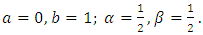 this gives the midpoint method.Another choice can be
 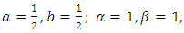 which give the modified Euler.Still another possibility is
 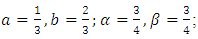 this is said to give a minimum bound to the error. All of these are special cases of second-order of Runge-Kutta methods.Fourth-order Runge-Kutta methods are most widely used and are derived in similar fashion.Greater complexity results from having to compare terms through
  and this gives a set of 11 equations in 13 unknowns. The set of 11 equations can be solved with 2 unknowns being chosen arbitrarily. The most commonly used set of values leads to the procedure;
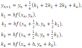 | (3.8) |
This Runge-Kutta method will be used to solve equation (1.1) in section 4. Numerically, we shall use Euler method and fourth-order Runge-Kutta method.
4. Results
Considering equation (1.1);Let  such that
  Therefore; equation (1.1) becomes;
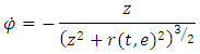 But from theorem 2, equation (3.5) states;
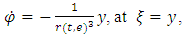 which is linear. (Hill’s type of equation at
  Euler method
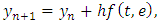
 Given
Given 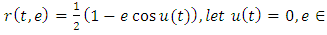
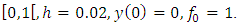
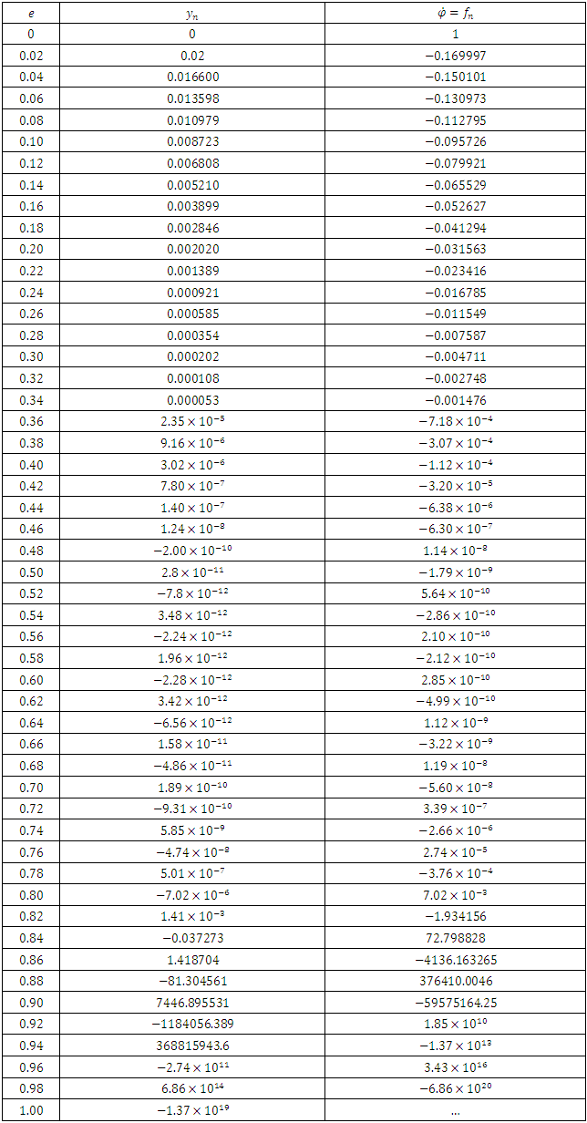
Table 1
 |
| |
|
The table above shows the results.Fourth-order Runge-Kutta methods: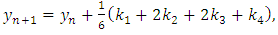 Using the same parameters, we obtain the results in the table below;
Table 2
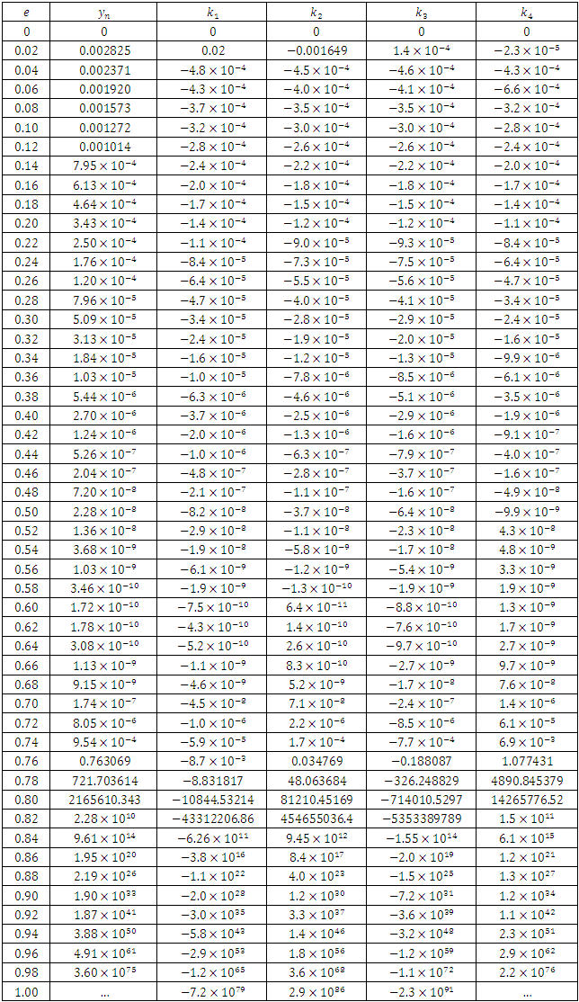 |
| |
|
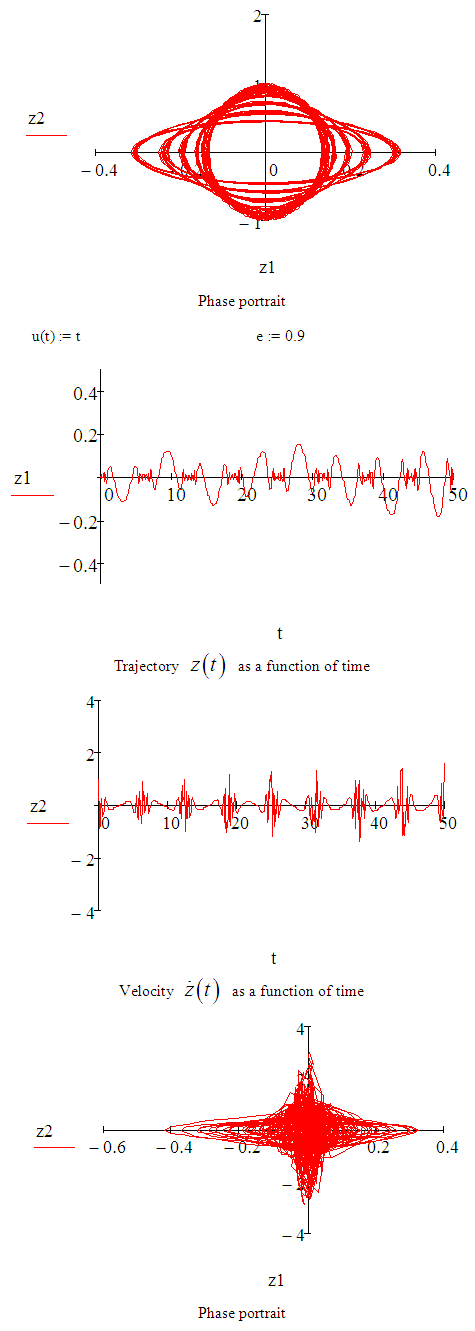
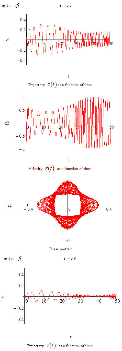
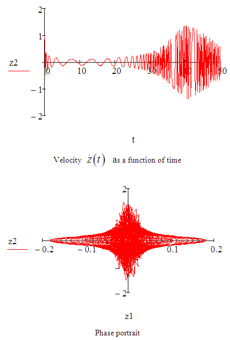
MATHCAD SIMULATIONSIMULATION OF 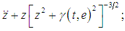

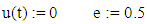 Define a function that determines a vector of derivative values at any solution point (t,Z):
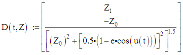 Define additional arguments for the ODE solver:
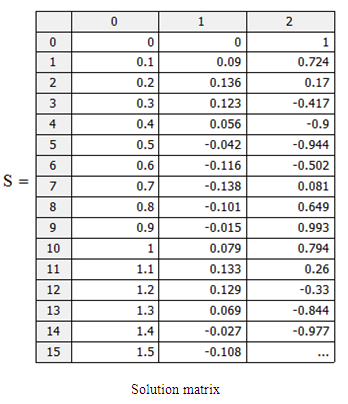
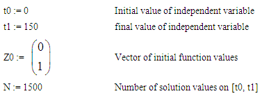 Solution matrix:
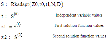
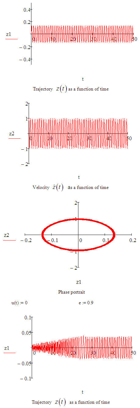
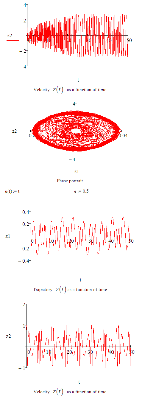
5. Conclusions
An approximate solution of the Sitnikov problem has been investigated using both the Euler and fourth-order Runge-Kutta methods. The fourth-order Runge-Kutta method gave us more accurate results than Euler method. The various values of eccentricities were obtained and demonstrated by simulations using MATCAD. The simulations reveal the behaviour of the solutions at any given eccentricity, this showed that the range for the search of eccentricities can be narrowed down at different values of eccentricities, different sinusoidal frequencies were obtained.
References
| [1] | L. Bakker and S. Simmons, A separating surface for Sitnikov-like n+1-body problems, J. Differential Equations 258 (2015), 3063-3087. |
| [2] | M. Corbera and J. Llibre, periodic orbits of the Sitnikov problem via a Poincare map, Celestial Mech. And Dynam. Astronom. 79 (2001), 97-117. |
| [3] | L. Jimenez-lara and A. Escalona-Buendia, Symmetries and bifurcation in the Sitnikov problem, Celestial Mech. And Dynam. Astronom. 79 (2001), 97-117. |
| [4] | J. Llibre and R.Ortega, On the families of periodic solutions of the Sitnikov problem, SIAM J. Appl. Dyn. Syst. 7 (2008), 561-576. |
| [5] | J. Moser, Stable and random motions in dynamical systems, Princeton University Press, Princeton, N. J., 1973. |
| [6] | R. Ortega and A. Rivera, Global bifurcation from the center of mass in the Sitnikov problem, Discrete Contin. Dyn. Syst. Ser. B 14 (2010), 719-732. |
| [7] | R. Ortega, Symmetric periodic solutions in the Sitnikov problem, Arch. Math. 107 (2016), 405-412. |
| [8] | E. Belbruno, J. Llibre and M. Ollé, On the families of periodic orbits which bifurcate from the circular Sitnikov motions, Celestial Mechanics and Dynamical Astronomy, 1994, 60(1): 99-129. |
| [9] | P. Rabinowitz, Some global results for nonlinear eigenvalue problems, J. Funct. Anal., 7(1971), 487-513. |

 Abstract
 Reference
 Full-Text PDF
 Full-text HTML