Pallavi P. Chopade1, Prabha S. Rastogi2
1Research Scholar, JJTU, Rajasthan, India
2Department of Mathematics, JJTU, Rajasthan, India
Correspondence to: Pallavi P. Chopade, Research Scholar, JJTU, Rajasthan, India.
| Email: |  |
Copyright © 2018 The Author(s). Published by Scientific & Academic Publishing.
This work is licensed under the Creative Commons Attribution International License (CC BY).
http://creativecommons.org/licenses/by/4.0/

Abstract
In this paper, effective algorithms of finite difference method (FDM) and finite element method (FEM) are designed. The solution of partial differential 2-D Laplace equation in Electrostatics with Dirichlet boundary conditions is evaluated. The electric potential over the complete domain for both methods are calculated. The developed numerical solutions in MATLAB gives results much closer to exact solution when evaluated at different nodes. An error analysis is also presented where the numerical error based on the L2 norm is computed. This error reduces monotonically by reducing the mesh size.
Keywords:
Finite difference method, Finite element method, Dirichlet boundary conditions, Laplace equation, Partial differential equation, Electrostatics
Cite this paper: Pallavi P. Chopade, Prabha S. Rastogi, Numerical Method Algorithms for Solution of Two-Dimensional Laplace Equation in Electrostatics, American Journal of Computational and Applied Mathematics , Vol. 8 No. 4, 2018, pp. 65-69. doi: 10.5923/j.ajcam.20180804.01.
1. Introduction
In the field of mathematics, formulation of differential equations and their respective solutions are the most important aspects to almost every numerical. They are also equally useful and important in many fields of engineering e.g. heat transfer, stress equation for beam, electromagnetic theory, etc.The exact solution of partial differential equation is difficult and complex. For problem involving irregular shapes, boundary conditions, material properties, etc. numerical methods such as finite difference method, finite element method, etc are best suited to provide approximate but acceptable values of unknown quantities at discrete number of points in the given domain. Instead of solving the problem for entire domain in one step, the solutions are obtained for each constituent unit and eventually combined to obtain the complete solution.Finite Difference Method and Finite Element Method were used extensively to analyze the stresses in various load conditions. Besides instrumental in structural analysis, they have been popularly used to solve differential and integral equations involved in various domains of Mechanical Engineering, Civil Engineering and Electronics Engineering. In electrostatics, Poisson or Laplace equation are used in calculations of the electric potential and electric field [1].A static electric field E in vacuum due to volume charge distribution when expressed in partial differential equations is given as  | (1) |
Equation 1 is Gauss’s law in a differential form.In cartesian co-ordinate system the del operator  is given by,
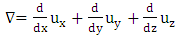 | (2) |
The static electric field in terms of gradient and scalar electric potential V is given by  | (3) |
On combining equation 1 and 3 | (4) |
where  is Laplacian operator.Equation 4 is termed as Poisson’s equation in electrostatics [2-3].The charge density
  in the region of interest when becomes zero, equation 4 becomes Laplace equation as [4],
 | (5) |
In cartesian coordinate system,  operating on electric potential
  for a two -dimensional Laplace equation is given as [5],
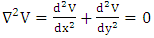 | (6) |
The solution of equation (6) is obtained using finite element method.The rest of the paper is organized into three sections. Section 2 defines the electrostatic 2-D problem and its formulation. Section 3 discusses numerical methods and exact solution for the given boundary value problem and calculates the accuracy of the developed algorithms and finally section 4 concludes the paper.
2. Problem Definition and Formulation
An infinitely long rectangular box with metallic walls having dimensions  as shown in Figure 1.1 is considered [1]. The bottom and vertical walls are maintained at zero electric potential while the top wall, separated by tiny slits, has fixed electric potential
  . Using numerical methods, find and compare the solutions of Laplace equation with exact solution and calculate the error. Plot the electric potential distribution. The Dirichlet boundary conditions
  .
.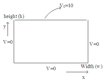 | Figure 1.1. A Rectangular region with metallic walls with boundary conditions |
A simple case of electric potential in infinite long rectangular box with metallic walls can be formulated in two-dimension Laplace equation as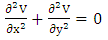 | (7) |
For the given problem,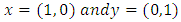 where
where  is the electric potential distribution in the domain and the Dirichlet boundary conditions are,
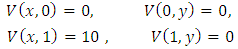 The rectangular region is divided into finite number of elements with every node and side being common with neighboring elements excluding the sides on the boundaries.
2.1. Finite Difference Method
The finite difference method (FDM) is a simple numerical approach used in numerical involving Laplace or Poisson’s equations.A numerical is uniquely defined by three parameters:1. Partial differential equation such as Laplace's or Poisson's equations.2. A solution domain3. Boundary and/or initial conditions.The solution to such numerical can be found using finite difference method that evaluates by discretizing the domain into a grid of nodes, approximates the differential equation with boundary condition by set of linear equations known as difference equation and solving these set of equation by either band matrix method or iteration method.A 2D domain along with boundary conditions i.e. electric potential divided into rectangular grid of 121 nodes with numbering is shown in figure 1.2(a).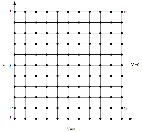 | Figure 1.2(a). Rectangular region with 10 x 10 grid for Finite Difference Method |
The FDM algorithm developed in MATLAB consists of following steps [12]• Step 1: Specify array size and boundary conditions• Step 2: Calculate step size and specify charge density, if needed.• Step 3: Specify boundary conditions.• Step 4: Use central difference method to calculate potential distribution and iterate it until all the values are achieved.• Step 5: Plot the results.
2.2. Finite Element Method
A nodal FEM when applied to a 2D boundary value problem in electromagnetics usually involves a second order differential equation of a single dependent variable subjected to set of boundary conditions. These boundary conditions can be of the Neumann type, the Dirichlet type, or the mixed type. The 2D geometry of the domain can be of arbitrary shape. An accurate illustration of this domain can be achieved using discretization techniques with either triangular or quadrilateral shapes called finite elements [6], [7].The solution of such 2-D boundary value problems using FEM can be solved using following steps [8-10]:a) 2D domain Discretization.b) Derivation of the weak formulation of the governing differential equation.c) Proper choice of interpolation functions.d) Derivation of the element matrices and vectors.e) Assembly of the global matrix system.f) Imposition of boundary conditions.g) Solution of the global matrix system.h) Postprocessing of the results.A 2D region domain denoted by ‘D’ on discretization gives 121 global nodes numbered through 1 to 121 and 200 equal triangular finite elements as shown in Figure 1.2(b). | Figure 1.2. Rectangular region with 10 x 10 grid Finite element mesh using triangular elements |
2.3. Exact Solution
The Laplace’s equation’s (Equation 1) solution to the given numerical, when subjected to Dirichlet boundary conditions,  is given by,
 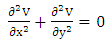 | (8) |
and can be analytically solved using variable separable form.The exact solution of electric potential as a function of x and y inside the for the given 2D rectangular domain is given by, 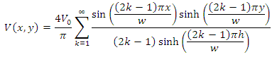 | (9) |
3. Numerical Solution for 2D Electrostatic Boundary Value Problem
The given 2D electromagnetic boundary value problem is solved using FDM and FEM algorithms developed in MATLAB and are compared with exact solution for the different nodes. The L2 norm error is also calculated and is given by,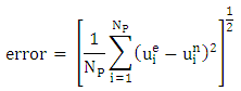 | (10) |
where  denoted the exact analytical solution at a particular point on grid,
  correspond the numerical solution at the same point, and
  represents the total number of points where the two solutions are evaluated.
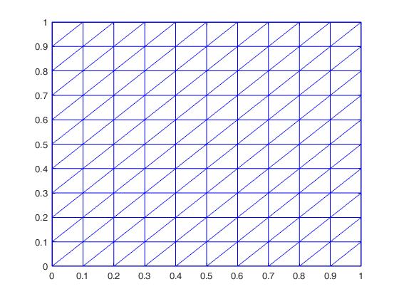 | Figure 1.3. Rectangular mesh of 10 x 10 grid in MATLAB |
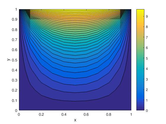 | Figure 1.4. Contour plot of the electric potential distribution inside the box (analytical solution) |
The FEM algorithm developed and implemented in MATLAB can be briefly described as,The FEM algorithm developed in MATLAB consists of following steps [10-11]Step 1: A Rectangular Geometry is definedStep 2: Define the number of elements in the x and y directionsStep 3: Define the given Electric potential i.e. top sideStep 4: Generate and plot the triangular mesh for given nodes/elementsStep 5: Define the overall boundary conditionsStep 6: Initialize the global K matrix and right-hand side vectorStep 7: Form and assemble the element matrices vectors into the global K matrix and right -hand side vectorStep 8: Apply Dirichlet boundary conditionsStep 9: Obtain the solution of the global matrix system and plot it Step 10: Find Exact Analytical Solution and evaluate the L2 norm error The comparison of electric potential at nodes evaluated using FDM and FEM developed in MATLAB and exact solution is shown in Table 1.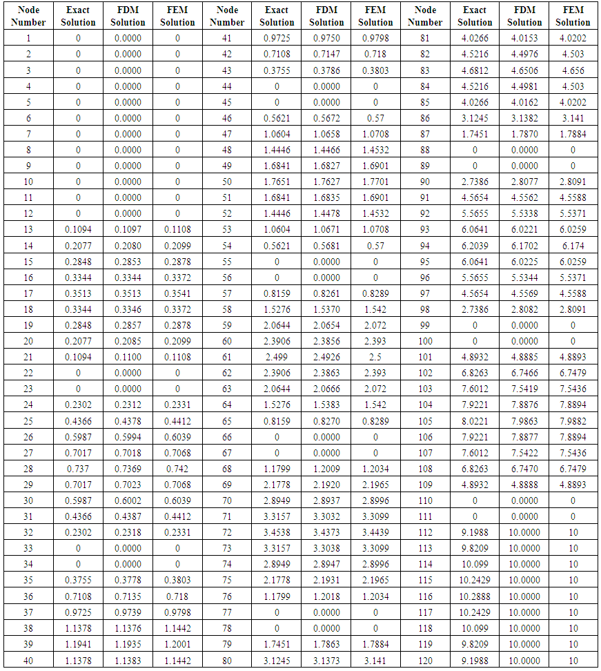 | Table 1. Comparison of numerical solutions with exact solution |
The graphical representation of FEM and exact solution is shown in Figure 1.5.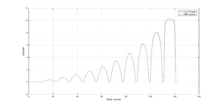 | Figure 1.5. Graphical representation of comparison of two solutions |
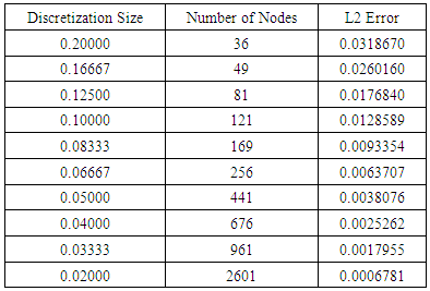
The accuracy of the numerical solution (FEM) developed in MATLAB is evaluated and is found to be 0.0128589.Similarly, the error as a function of mesh size is calculated as shown in Table 2 and is graphically represented in figure 1.6.Table 2. Discretization size and Numerical error based on the L 2 norm
 |
| |
|
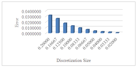 | Figure 1.6. Discretization size vs Numerical error based on the L2 norm |
4. Conclusions
This paper presents numerical techniques to solve two-dimensional differential equation system for electrostatic field of engineering with Dirichlet boundary conditions. The electrical potential over the complete domain is evaluated. The FDM and FEM solutions give closer results to exact solution at different nodes.It is observed that by increasing the number of elements the FEM solution approaches to exact solution, thus reducing the numerical error, monotonically. Additionally, by using higher order interpolation functions, an accurate solution can be obtained thus reducing the numerical error substantially.
References
| [1] | Lonngren, K.E., Savov, S.V. and Jost, R.J., 2007. Fundamentals of Electromagnetics with MATLAB. Scitech publishing. |
| [2] | Papanikos, G. and Gousidou-Koutita, M.C., 2015. A Computational Study with Finite Element Method and Finite Difference Method for 2D Elliptic Partial Differential Equations. Applied Mathematics, 6(12), p.2104. |
| [3] | Chaudhari, T.U. and Patel, D.M., 2015. Finite Element Solution of Poisson’s equation in a homogeneous medium. |
| [4] | Brenner, S. and Scott, R., 2007. The mathematical theory of finite element methods (Vol. 15). Springer Science & Business Media. |
| [5] | Mrs. Pallavi P. Chopade, Dr. Prabha S. Rastogi "Formulation of Finite Element Method for 1-D Poisson Equation", International Journal of Mathematics Trends and Technology (IJMTT). V56(5): 360-365 April 2018. ISSN: 2231-5373. |
| [6] | Sharma, N., Formulation of Finite Element Method for 1D and 2D Poisson Equation. |
| [7] | Agbezuge, L., 2006. Finite Element Solution of the Poisson equation with Dirichlet Boundary Conditions in a rectangular domain. |
| [8] | Jain, M.K., 2003. Numerical methods for scientific and engineering computation. New Age International. |
| [9] | Rao, N., 2008. Fundamentals of Electromagnetics for Engineering. Pearson Education India. |
| [10] | Sadiku, M.N., 2011. Numerical techniques in electromagnetics with MATLAB. CRC press. |
| [11] | Yang, W.Y., Cao, W., Chung, T.S. and Morris, J., 2005. Applied numerical methods using MATLAB. John Wiley & Sons. |
| [12] | Mitra, A.K., 2010. Finite difference method for the solution of Laplace equation. Department of aerospace engineering Iowa state University. |

 Abstract
 Reference
 Full-Text PDF
 Full-text HTML