1. Introduction

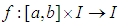
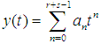
It is no exaggeration to say that differential equations play important roles in modeling of physical and engineering problems, such as those in solid and fluid mechanics, viscoelasticity, biology, physics and many other areas, [1]. The theory of Fuzzy Differential Equations (FDEs) has focused much attention in the last decades since it provides good models for dynamical systems under uncertainty, [2].

In general, the parameters, variables and initial conditions within a model are considered as being defined exactly. In reality, there may be only vague, imprecise or incomplete information about the variables and parameters available. This can result from errors in measurement, observation, or experimental data; or maintenance induced errors. To overcome uncertainties or lack of precision, one can use a fuzzy environment in parameters, variables and initial conditions in place of exact (fixed) ones by turning general differential equations into FDEs.

In real applications, it can be complicated to obtain exact solution of FDEs due to the complexities in fuzzy arithmetic, creating the need for use of reliable and efficient numerical techniques in the solution of FDEs. Thus, there are many methods that have been derived to study FDEs. The first and most popular approach is using Hukuhara differentiability for fuzzy number value functions. Here, the existence and uniqueness of solutions of FDEs are analyzed. Under appropriate conditions, the FDEs that will be considered have locally two solutions. Some methods that exist in literature for the solutions of FDEs under the Hukuhara differentiability concept include Adomian decomposition method [3, 4], modified Euler’s method [5], Improved Runge-Kutta method [6], He’s homotopy perturbation method [7], Simpson’s rule [8], Picard method [9], Combined Laplace transformation and variational iteration methods [10], among others.

Of recent, some results have been published on random FDEs. The random approach can be adequate in modeling of the dynamics of real phenomena which are subjected to two kinds of uncertainty: randomness and fuzziness simultaneously, [2]. Also, according to [5], the study of FDEs forms a suitable setting for mathematical modeling of real-world problems in which uncertainties or vagueness pervade.

In this research, we shall be interested in the analysis and computation of FDEs of the form

(1)

where is a fuzzy function of is a fuzzy function of the crisp variable and the fuzzy variable is the fuzzy derivative of and is a triangular or a triangular shaped fuzzy number.

The sufficient conditions for the existence of a unique solution to the FDE (1) are that be continuous function satisfying the Lipschitz condition,

(2)

We replace the interval by a set of discrete equally spaced grid points

2. Preliminaries

In this section, some definitions shall be presented. We shall also introduce some necessary notations that shall be employed in this paper.

Consider the space of dimensional real numbers and let be the space of nonempty compact and convex sets of . If , denote the set of (closed bounded) intervals of the real line. Let be the set of all upper semi-continuous normal convex fuzzy numbers with bounded level intervals. Then, is the set of all triangular or triangular shaped fuzzy number and .

Definition [11]

A fuzzy number is a fuzzy subset of the real line with normal, convex and upper semi continuous membership function of bounded support. A fuzzy number is represented by an ordered pair of functions which satisfies the following three conditions:

(i) is a bounded left continuous non-decreasing function

(ii) is a bounded right continuous non-increasing function

(iii)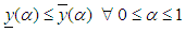

A fuzzy number is a generalization of a regular, real number in the sense that it does not refer to one single value but rather to a connected set of possible values, where each possible value has its own weight between 0 and 1. This weight is called the membership function.

It is important to state that our fuzzy number will be triangular shaped. A triangular fuzzy number is defined by three real numbers , where the base of the triangle is the interval and its vertex is at .

Triangular fuzzy numbers will be written as The membership function for the triangular fuzzy number is defined as

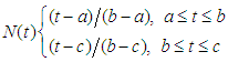(3)

For a fuzzy number to be triangular shaped, we require the graph of the corresponding membership function to be continuous and

(i) monotonically increasing on

(ii) momotonically decreasing on

also, the core of a fuzzy number is the set of values where the membership value equals one, [12].

Definition [5]

Let be a nonempty set. A fuzzy set in is characterized by its membership function . Then is interpreted as the degree of membership of an element in the fuzzy set for each Definition [13]

The generalized Hukuhara difference of two sets (difference for short) is defined as follows,

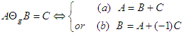(4)

Definition [5]

Let and be such that , then the gH-derivative of a function can be defined as

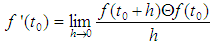(5)

If satisfying (5) exists, we say that is generalized Hukuhara differentiable (differentiable for short) at . It is important to state that sometimes, may be strongly generalized (Hukuhara) or weakly generalized (Hukuhara) differentiable at .

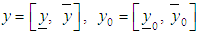
We denote the fuzzy function by where are lower and upper branches of

Definition [14]

Let be a real interval. A mapping is called a fuzzy process and we define its level set as

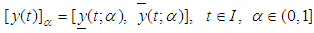(6)

Definition [14]

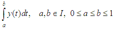The fuzzy integral is defined by

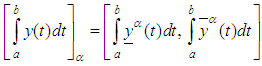(7)

provided that the Lebesque integrals on the right exist.

Note that if is Hukuhara differentiable and its Hukuhara derivative is integrable over then,

(8)

for all values of where

Definition [15]

A numerical integration scheme is said to be -stable for some if the wedge

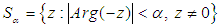(9)

is contained in its region of absolute stability. The largest is called the angle of absolute stability.

3. Interval Differential Equations and the Generalized Hukuhara Differentiability

According to [13], generalization of the concept of Hukuhara differentiability can be of great help in the study of IDEs. Consider the IDE

(10)

where with,

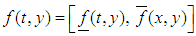for

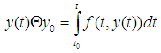
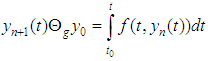
Lemma 3.1 [13]

The IDE (10) is locally equivalent to the integral equation

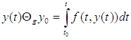(11)

The existence of gH-difference imply that the integral equation in (11) is actually a unified formulation for one of the integral equations

and

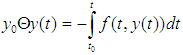with being the classical Hukuhara difference.

This integral equation formulation helps us in obtaining existence result for IDEs.

Theorem 3.1 [13]

Let 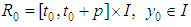nontrivial and be continuous. If satisfies the Lipchitz condition , then the interval problem (10) and by extension the FDE (1) has exactly two solutions 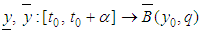satisfying

More precisely, the successive iterations

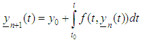and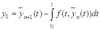

converge to these two solutions respectively.

See [13] for proof.

4. Derivation of a Computational Method and Analysis of Its Basic Properties

In order to compute the approximate solution to FDEs of the form (1), we derive a highly efficient two-step computational method that has the form,

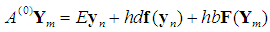(12)

and also analyze its basic properties like order, convergence, consistence and stability region.

The derivation is carried out using power series basis function of the form,

(13)

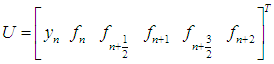
where are the numbers of collocation and interpolation points respectively.

Let the approximate solution to FDE (1) be given by power series of degree 5; taking in equation (13) gives,

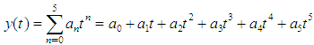(14)

Differentiating equation (14), we get

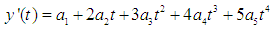(15)

Substituting (15) into (1) gives,

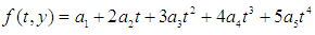(16)

Interpolating (14) at point and collocating (16) at points , leads to a system of nonlinear equation of the form,

(17)

where

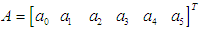
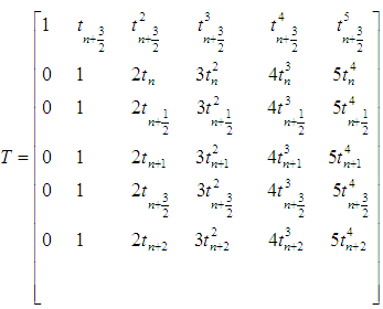Solving the system (17) by Gauss elimination method for the and substituting back into the power series basis function gives a linear multistep method of the form,

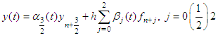(18)

where the coefficients of are given by,

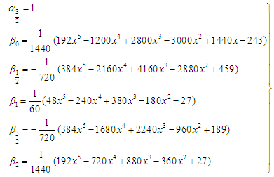(19)

and is given as

(20)

Evaluating (18) at gives a discrete two-step computational method of the (12) given by,

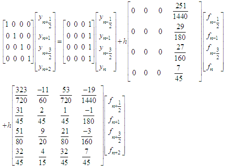(21)

Some basic properties of the computational method derived are analyzed below:

(i) The order of the computational method and error constants are given respectively by 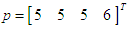and

(ii) The method is adjudged to be consistent since it has order . Note that consistency controls the magnitude of the local truncation error committed at each stage of the computation, [16]

(iii) The computational method is said to be zero-stable, if the roots of the first characteristic polynomial defined by 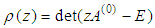satisfies and every root satisfying have multiplicity not exceeding the order of the differential equation, [16, 17]. The first characteristic polynomial is given by,

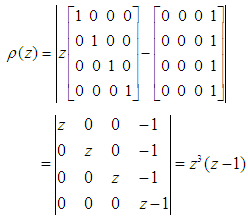Thus, solving for in

(22)

gives . Hence, the computational method (21) is said to be zero-stable.

(iv) The computational method is convergent since it is consistent and zero-stable.

(v) The region of absolute stability of the computational method is shown in the figure below

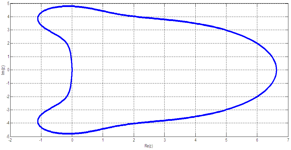Figure 4.1. Stability region of the computational method

The stability region obtained in Figure 4.1 is -stable, since the stability region consists of the complex plane outside the enclosed figure. Note that the unstable region is the interior of the curve (when the curve is on the positive plane) while the stability region contains the exterior part of the curve.

5. Results

Let and denote respectively the exact (analytic) solution and approximate (computed) solution of the fuzzy differential equations of the form (1). That is,

Also, let absolute error be defined by

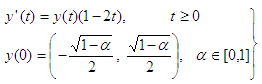
We shall apply the computational method derived on some FDEs to test its efficiency and reliability. It is important to state that the FDEs that shall be solved in this section are all interval differential equations.

Problem 5.1:

Consider the Fuzzy differential equation,

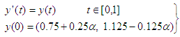(23)

The exact solution is given by,

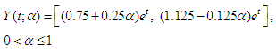(24)

The exact solution is computed at

Source: [18]

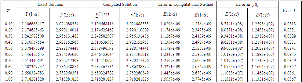Table 5.1. Showing the result for Problem 5.1 at t = 1

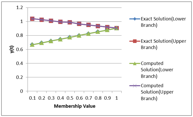
Figure 5.1. Graphical results comparing the exact and computed solutions for Problem 5.1

Problem 5.2:

Consider the Fuzzy differential equation,

(25)

The exact solution is given by,

(26)

The exact solution is computed at

Source: [6]

Table 5.2. Showing the comparison of absolute errors of our computational method with that of [6] at t = 0.1 for Problem 5.2

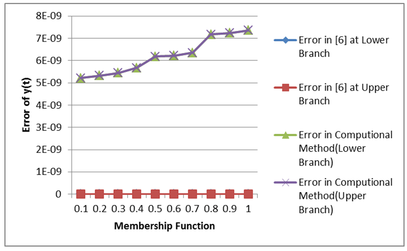Figure 5.2. Graphical results comparing the absolute errors in the computational method with that of [6] for Problem 5.2

Problem 5.3:

Consider the Fuzzy differential equation,

(27)

The exact solution is given by,

(28)

The exact solution is computed at

Source: [18]

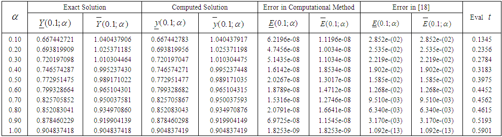Table 5.3. Showing the result for Problem 5.3 at t = 0.1

Figure 5.3. Graphical results comparing the exact and computed solutions for Problem 5.3

From the results presented in Tables 5.1 to 5.3, it is clear that the computational method derived is efficient and reliable in approximating the solution to fuzzy differential equations of the form (1). We observed that the results obtained show that the method derived perform better that the ones with which we compared our results with. The evaluation time per seconds obtained were also observed to be very small, showing that the computational method generates results very fast. The graphical results presented in Figures 5.1 and 5.3 further buttress the fact that the exact and computed solutions converge for Problems 5.1 and 5.3. For Figure 5.2, it is clear that the error in the computational method is by far smaller than that of [6] for Problem 5.2.

6. Conclusions

IDEs with a generalized Hukuhara type differentiability were studied to obtain an existence theorem and uniqueness of two solutions for FDEs. Special case interval differential equations called the fuzzy differential equations have been studied. We also looked at the influence of Hukuhara differentiability on such differential equations. It is however important to state that the setback of this approach is that the solution becomes fuzzier as time goes by. Thus, the fuzzy solution behaves quite differently from the crisp solution. To avoid this setback, [19] interpreted FDEs as a family of differential inclusions. However, the main shortcoming of using differential inclusions is that we do not have a derivative of a fuzzy-number-valued function, [5].

In view of these shortcomings, the generalized differentiability was introduced in [20, 21, 22] where the original initial value problem is replaced by two parametric ordinary differential systems which are then solved numerically using classical algorithm. You may refer to the work of [23], where they applied the block backward differentiation formula under generalized differentiability.

Conclusively, one may also say that the computational method adopted in this research effectively approximates the FDEs.