M. Tahmina Akter1, 2, M. A. Mansur Chowdhury2
1Department of Mathematics, Chittagong University of Engineering & Technology, Chittagong, Bangladesh
2Jamal Nazrul Islam Research Center for Mathematical and Physical Sciences, University of Chittagong, Chittagong, Bangladesh
Correspondence to: M. Tahmina Akter, Department of Mathematics, Chittagong University of Engineering & Technology, Chittagong, Bangladesh.
| Email: |  |
Copyright © 2017 Scientific & Academic Publishing. All Rights Reserved.
This work is licensed under the Creative Commons Attribution International License (CC BY).
http://creativecommons.org/licenses/by/4.0/

Abstract
The Variational Iterational Method has been successfully applied to solve many nonlinear differential equations. Recently this method has been used to solve quantum mechanical problems. To fulfill this goal we have tried to use this method for solving a coupled Schrödinger-Klein-Gordon equation. We have considered a system of coupled Schrödinger-Klein-Gordon equation with appropriate initial condition then we have applied the Variational Iterational Method for finding analytical solutions of these equations. The numerical solutions of coupled Schrödinger- Klein-Gordon equation have been represented graphically. These results are significant which shows the efficiency of the proposed algorithm. It is now apparent that Variational Iterational Method is more efficient and easier to handle as compare with other method like as the Modified Decomposition Method.
Keywords:
Variational Iteration Method, Coupled Schrödinger-Klein-Gordon Equation, Lagrange Multiplier, Variational Theory
Cite this paper: M. Tahmina Akter, M. A. Mansur Chowdhury, Variational Iteration Method for Solving Coupled Schrödinger-Klein-Gordon Equation, American Journal of Computational and Applied Mathematics , Vol. 7 No. 1, 2017, pp. 25-31. doi: 10.5923/j.ajcam.20170701.03.
1. Introduction
In non-relativistic case the motion of a particle in a force field can be described in terms of a differential equation which is called Schrödinger wave equation. It is a highly non-linear differential equation. The equation consists of a kinetic energy term and a potential energy terms. So its solution depends on the potential energy of the particle taken into consideration. The prototype equation in relativistic case is called Klein-Gordon equation which is even more complicated than the Schrödinger wave equation. Here the relativistic effect is included. This means that the spin of the particle are included. However, after various analysis it is found that this Klein-Gordon equation describes only the motion of the spin zero particle. That is like  -meson and so on. For spin half particle such as electron, proton and etc. another wave equation is developed by Dirac which is called Dirac equation. All of these equations are highly non-linear and so is extremely difficult to get an exact solution. Researchers have been trying to solve these equation considering various types of potentials and assumptions.In this article we tried to solve Schrödinger- Klein-Gordon Equation numerically. Recently J.H. He developed a numerical method called variational iterational method (VIM) which is more effective and applicable in variety types of non-linear equations. We have applied this method in solving different types of non-linear differential equations. Many others also used this method to study the linear wave equation, non-linear wave equations and wave-like equation in bounded and unbounded domains.The variational iterational method (VIM) developed in 1999 by J. H. He in [1-3] which he used to study the linear wave equation, nonlinear wave equation and wave-like equation in bounded and unbounded domains. The method has been proved by many authors to be reliable and efficient for a wide variety of scientific applications, linear and nonlinear as well. The Schrödinger– Klein-Gordon (SKG) equation is a kind of nonlinear evolution equation. We know the particles can be identified in dual way. That means it is either particle like or wave like. So if we can find the behavior of a wave phenomena it will lead us to identify with the particle. That is why any kind of solution of SKG equation will play an important role in quantum field theory. The Schrödinger– Klein-Gordon (SKG) equation is
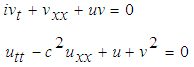 | (1) |
Where  We will solve this equation using VIM. In this method, general Lagrange multipliers are introduced to construct correction functional for the problems. The multipliers can be identified optimally via the variational theory. There is no need of linearization or discretization and large computational work and round-off errors is avoided. It has been used to solve effectively, easily and accurately a large class of nonlinear problems with approximation [6-13]. The main goal of the present study is to find the analytic solutions of the coupled Schrödinger– Klein-Gordon [4, 5] by the variational iteration method and compare with the Modified Decomposition Method and finally to see the behaviour of the solution by three dimensional and corresponding two dimensional figure for real and imaginary parts of that solutions.
2. Description of Variational Iteration Method (VIM)
The variational iteration method (VIM) can be explained briefly in the following way. Let us consider the following general nonlinear partial differential equation: | (2) |
Where A is a differential operator with nonlinear terms and g(t) is a known function. We can separate A into linear and nonlinear parts. That is let us rewrite equation (2) in the following way: 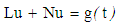 where L is a linear operator, N is a nonlinear term and g(t) is a known function. To solve this type of nonlinear differential equation J.H. He proposed the variational iteration method whose brief description is the following, He said to solve equation (2) let us consider the following iteration formula
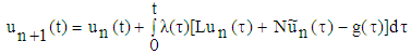 | (3) |
which is also called correction functional for equation (2), where  is a general Lagrange multiplier which can be identified optimally via variational theory,
  is considered as restricted variations i.e.
  . It is required first to determine the Lagrangian multiplier
  that will be identified optimally via integration by parts. The successive approximation
 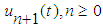 of the solution
  will be readily obtained upon using the Lagrangian multiplier obtained and by using any selective function u0. The initial values
  and
and  are usually used for the selective zeroth approximation of u0. Having
  determined then several approximation
  can be determined. Consequently, the solution is given by
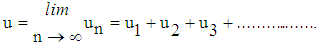 | (4) |
It is worth mentioning here that different types of linear or nonlinear equations will give rise to different values for the Lagrange multiplier  . This method is used in the next section to solve equation (1).
3. Numerical Solution of Schrödinger– Klein-Gordon Equation
In this section, we first consider the coupled Schrödinger– Klein-Gordon (SKG) equation with the initial conditions [4, 5] then tried to solve the solutions of these coupled equations by using the VIM. The coupled system of SKG is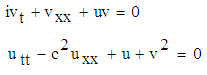 | (5) |
And the initial conditions are 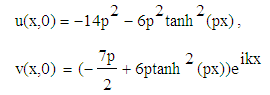 | (6) |
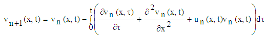
where p and k are arbitrary constants and also considering 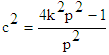 for the coupled SKG equations (5) with initial conditions (6).In order to obtain VIM solution of the equation (5) with initial conditions (6) we construct a correction functional which reads
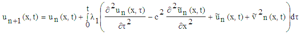 | (7) |
 | (8) |
where  and
and are the general Lagrange multipliers and
  ,
,  denote restricted variations, i.e.
 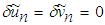 . Its stationary conditions can be obtained as follows
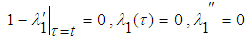 | (9) |
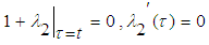 | (10) |
The Lagrange multipliers can therefore be identified as  and
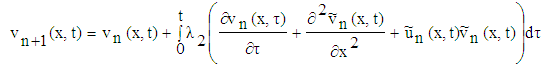
and  and the variational iteration formula is obtained in the form of:
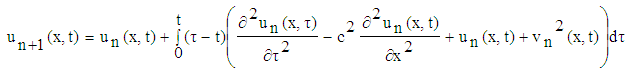 | (11) |
 | (12) |
Using the initial conditions we can solve equations (11) and (12) to get the solutions u(x,t) and v(x,t) which are :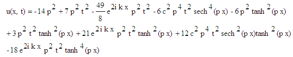 | (13) |
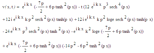 | (14) |
In the same manner using the iteration formulas (11) and (12) we can obtain the higher order approximations of equation (5).
4. Numerical Results and Discussions
In the present numerical computation we have assumed  ,
, and
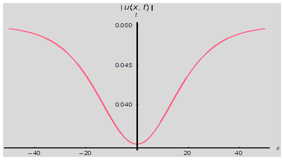
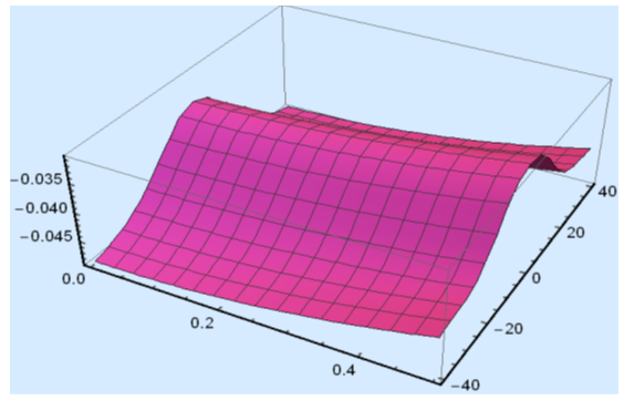
and  For numerical result equations (13) and (14) have been used to draw the graphs as shown in figures 1(a), 2(a), 3(a), 4(a) and so on and corresponding two dimensional graphs as 1(b), 1(c), 2(b), 2(c), 3(b), 3(c), 4(b), 4(c) and so on respectively. The approximated solution of absolute value of u(x,t) is plotted in figures 1(a) for
  and
and  and corresponding two dimensional graphs are drawn in figures 1(b) and 1(c) for
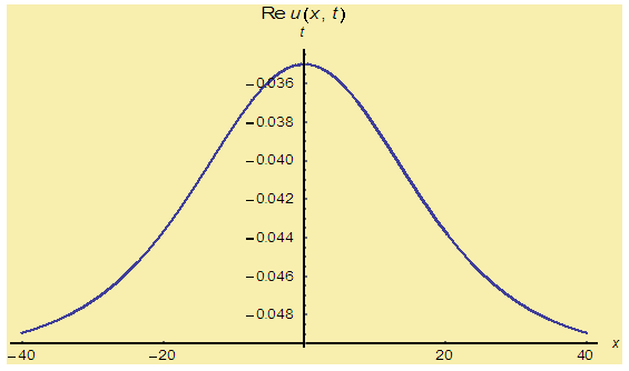
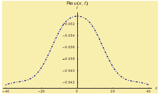
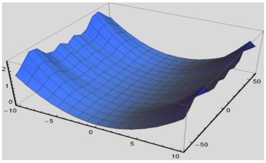
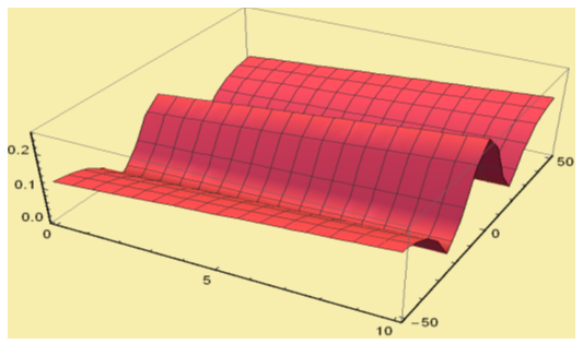
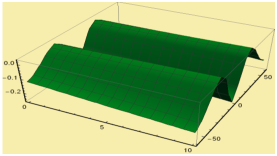
  and a fixed value t. Real value of u(x,t) are plotted in figures 2(a) and 3(a) for different ranges of variables x and t and corresponding two dimensional behaviours are shown in figures 2(b), 2(c) and 3(b), 3(c) for different fixed value of t. Also imaginary u(x,t) is plotted in figure 4(a) and in figures 4(b) and 4(c) are presented for corresponding 2D for a fixed value of t. In the same way the approximated solution of absolute, real and imaginary v(x,t) are plotted in Figs. 5(a), 6(a) and 7(a) for different ranges of variables x and t respectively. In Figs. 5(b), 5(c), 6(b), 6(c) and 7(b), 7(c) are shown their corresponding two dimensional graphs. Here we see that the behaviour of the solutions are unchanged for the fixed value of t.
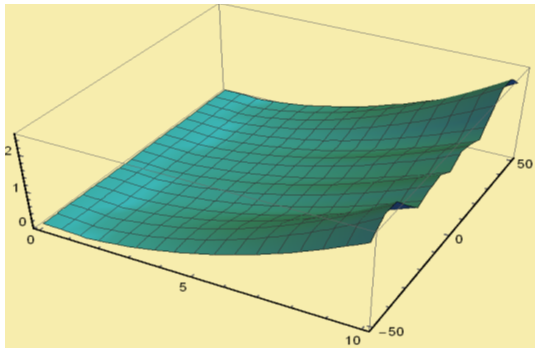 | Figure 1(a). Solution for Abs u(x,t) for  and and  |
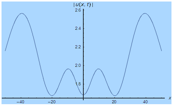 | Figure 1(b). Corresponding two dimensional graph for a fixed value  |
 | Figure 1(c). Corresponding two dimensional graph for a fixed value  |
 | Figure 2(a). Solution for Re u(x,t) for  and and  |
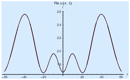
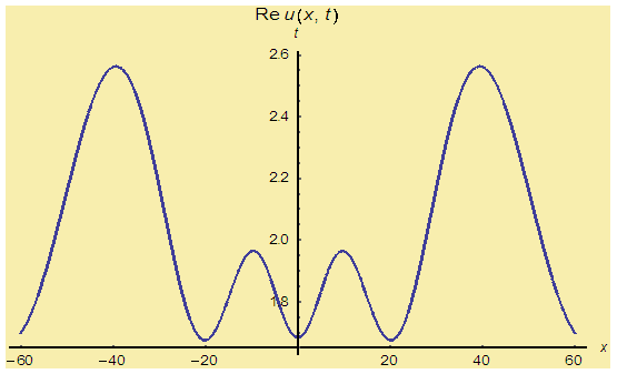
 | Figure 2(b). Corresponding two dimensional graph for a fixed value  |
 | Figure 2(c). Corresponding two dimensional graph for a fixed value  |
 | Figure 3(a). Solution for Re u(x,t) for  and and  |
 | Figure 3(b). Corresponding two dimensional graph for a fixed value  |
 | Figure 3(c). Corresponding two dimensional graph for a fixed value  |
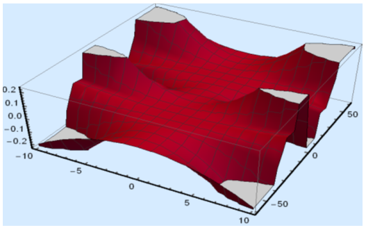 | Figure 4(a). Solution for Im u(x,t) for  and and  |
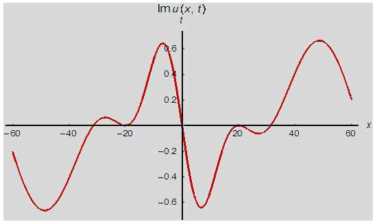 | Figure 4(b). Corresponding two dimensional graph for a fixed value  |
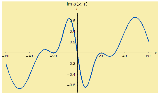 | Figure 4(c). Corresponding two dimensional graph for a fixed value  |
 | Figure 5(a). Solution for Abs v(x,t) for  and and  |
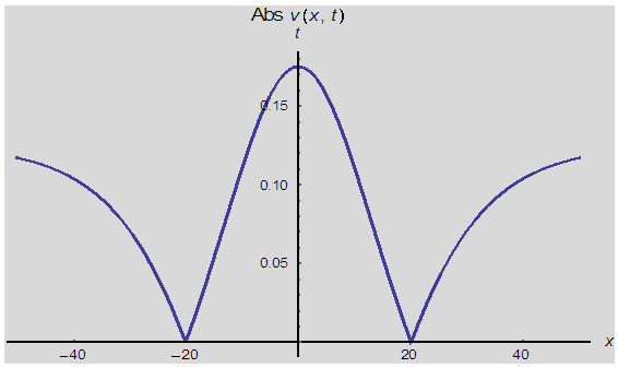 | Figure 5(b). Corresponding two dimensional graph for a fixed value  |
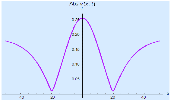 | Figure 5(c). Corresponding two dimensional graph for a fixed value  |
 | Figure 6(a). Solution for Re v(x,t) for  and and  |
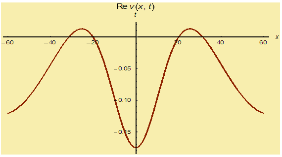 | Figure 6(b). Corresponding two dimensional graph for a fixed value  |
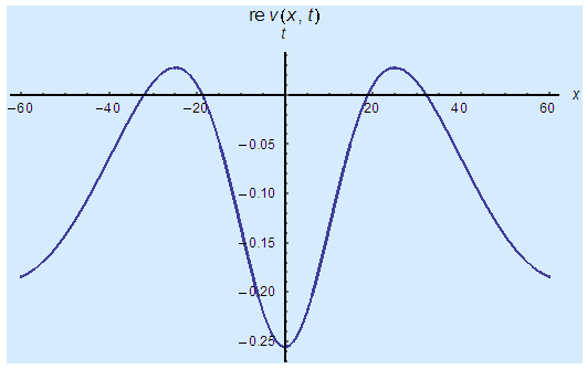 | Figure 6(c). Corresponding two dimensional graph for a fixed value  |
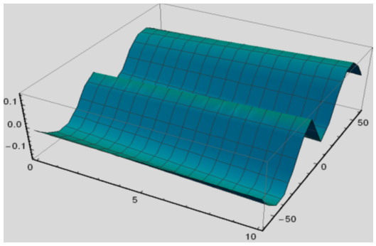 | Figure 7(a). Solution for Im v(x,t) for  and and  |
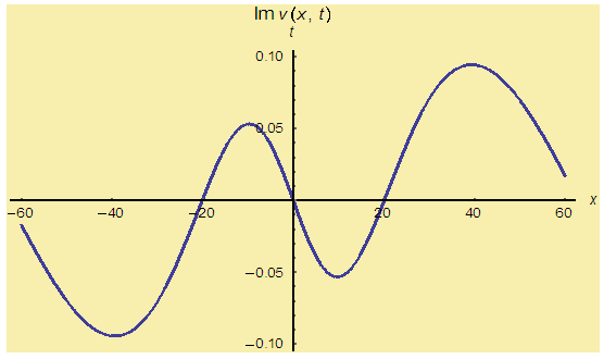 | Figure 7(b). Corresponding two dimensional graph for a fixed value  |
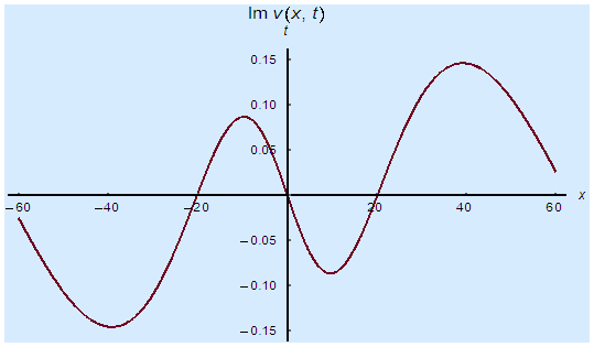 | Figure 7(c). Corresponding two dimensional graph for a fixed value  |
5. Conclusions
In this work, variational iteration method has been successfully applied for finding the approximate solution of the coupled Schrödinger Klein-Gordon equation. The numerical results obtained by VIM were observed to be in an excellent agreement with the results obtained by modified decomposition method. This indicates that the method is very efficient, reliable and experiences high accuracy. Moreover, unlike the traditional perturbation methods, VIM does not require any small parameter. In VIM we do not need discretization of time or space which reduces the computational errors and computer memory usage. The method is able to solve this nonlinear problem effectively and more easily as compared to other numerical techniques like adomain decomposition method. Due to its simplicity, flexibility and accuracy, VIM has been used to solve a wide range of linear and non-linear problems in science and engineering. Therefore, it provides more realistic series solutions that generally converge very rapidly in real physical problems.
References
| [1] | J.H. He, “Approximate solution of nonlinear differential equations with convolution product nonlinearities”, Comput. Methods Appl. Mech. Eng. 167 (12) (1998) 69–73. |
| [2] | J.H. He, “Approximate analytical solution for seepage flow with fractional derivatives in porous media”, Comput. Methods Appl. Mech. Eng. 167 (12) (1998) 57–68. |
| [3] | J.H. He, “Variational iteration method –a kind of non-linear analytical technique: some examples”, Int. J. Non-Linear Mech. 34 (4) (1999) 699–708. |
| [4] | A. Doosthoseini and H. Shahmohamadi, “Variational Iteration Method for solving couple Schrödinger-KdV Equation”, Applied Mathematical Sciences, Vol. 4, 2010, no. 17, 823-837. |
| [5] | S. S. Ray, “Solution of the Coupled Klein-Gordon Schrödinger Equation Using the Modified Decomposition Method”, International Journal of Nonlinear Science Vol. 4(2007) No.3, pp.227-234. |
| [6] | A. M. Wazwaz, “The decomposition method applied to systems of partial differential equations and to the reaction–diffusion Brusselator model”, Applied Mathematics and Computation, 110 (2-3), 251-264(2000). |
| [7] | A. M. Wazwaz, “Approximate solutions to boundary value problems of higher order by the modified decomposition method” Computers & Mathematics with Applications. 40 (6-7), 679-691(2000). |
| [8] | A. M. Wazwaz, “The modified decomposition method applied to unsteady flow of gas through a porous medium”, Applied Mathematics and Computation. 118(2-3), 123-132 (2001). |
| [9] | A. M. Wazwaz, “Construction of soliton solutions and periodic solutions of the Boussinesq equation by the modified decomposition method”, Chaos, Solitons & Fractals. 12(8), 1549-1556(2001). |
| [10] | A. M. Wazwaz, “Construction of solitary wave solutions and rational solutions for the KdV equation by Adomian decomposition method” Chaos, Solitons, & Fractals. 12(12), 2283-2293(2001). |
| [11] | A. M. Wazwaz, “A computational approach to soliton solutions of the Kadomtsev–Petviashvili equation”, Applied Mathematics and Computation. 123(2), 205-217(2001). |
| [12] | A. M. Wazwaz, Gorguis, A. “An analytic study of Fisher’s equation by using Adomian decomposition method”, Applied Mathematics and Computation. 154 (3), 609-620(2004). |
| [13] | A. M. Wazwaz, “Analytical solution for the time-dependent Emden–Fowler type of equations by Adomian decomposition method”, Applied Mathematics and Computation. 166(3), 638-651(2005). |
| [14] | E. Fan, “Multiple traveling wave solutions of nonlinear evolution equations using a unified algebraic method”, J. Phys. A 35 (2002) 6853–6872. |
| [15] | E. Yusufoglu, “Variational iteration method for construction of some compact and noncompact structures of Klein–Gorden equations”, Int. J. Nonlinear Sci. Numer. Simul. 8 (2) (2007) 153–158. |
| [16] | A. Darwish and E. G. Fan, “A series of New Explicit Exact Solutions for the Coupled Klein-Gordon-Schrodinger Equations” Chasos Soliton & Fractals. 20,609-617(2004). |
| [17] | S. Liu, Z. Fu and Z. Wang, “The Periodic Solutions for a Class of Coupled Nonlinear Klein-Gordon Equations” Physics Letters A. 323,415-420(2004). |

 Abstract
 Reference
 Full-Text PDF
 Full-text HTML