1. Introduction

This paper represents our attempt towards establishing the universal metric of the uncertainty value of micro- and macro-physics mathematical models by the application of information theory.

The very act of a measurement process already implies an existence of the formulated physical-mathematical model describing the phenomenon under investigation. Measurement theory focuses on the measurement process of experimentally determining the value of a quantity with the help of special technical means called measuring instruments [1]. It covers only aspects of the measuring procedure and data analysis of the observed or researched variable after formulating the mathematical model. So, the issue of uncertainty that exists before the beginning of the experiment or computer simulation and arising as a result of the limited number of variables recorded in the mathematical model is generally ignored in measurement theory.

In the scientific community the prevailing view is the more precise the instrument used for the model development, the more accurate the results, and the measurement uncertainty is also lower. Basically, in our everyday world it is possible to reduce the uncertainty in the determination of the studied process to a minimum. This, in turn, causes a widely held opinion that the usage of supercomputers, a huge number of simulations and large scale mathematical modeling can allow us to reach a high degree of accuracy of the model describing the observed material system [2-4]. For example, a standard input file of Energyplus as published by the US Department of Energy as a beta-testing of a whole-building simulation engine to describe a building has about 3,000 inputs. Its preliminary calculated uncertainty of, for example, room temperature, is very hard to estimate, because it strongly depends on the accuracy of the modeling inputs. Without measured data to compare and calibrate, energy simulation results can easily be 50–200% of the actual building energy use. For this reason it is not possible to validate a model and its results, but only to increase the level of confidence that is placed in them [5].

In contrast to the above-mentioned opinion, human intuition and experience suggests the simple, at first glance, truth. For a small number of variables, the researcher gets a very rough picture of the process being studied. In turn, the huge number of accounted variables can allow deep and thorough understanding of the structure of the phenomenon. However, with this apparent attractiveness, each variable brings its own uncertainty into the integrated (theoretical or experimental) uncertainty of the model or experiment. In addition, the complexity and cost of computer simulations and field tests increases enormously. Therefore, some optimal or rational number of variables that is specific to each of the studied processes must be considered in order to evaluate the physical-mathematical model. This work seeks to develop a fundamentally novel method to characterize the model firstborn uncertainty (model discrepancy [6]) connected only with the finite number of recorded variables. Of course, in addition to this uncertainty, the overall measurement inaccuracy includes the posterior uncertainties related to the internal structure of the model and its subsequent computerization: inaccurate input data, inaccurate physical assumptions, the limited accuracy of the solution of integral-differential equations, etc. Detailed definitions of many different sources of these uncertainties are outlined in the literature [1, 6-8].

The introduced novel analysis is intended to help physicists and designers to determine the most simple and reliable way to select a model with the optimal number of recorded variables calculated according to the minimum achievable value of the model uncertainty.

The present approach begins with the analysis of several publications related to usage of the concepts of "information quantity" and “entropy” for real applications in physics and engineering (Chapter 2), followed by the formulation of a system of dimensional variables, from which a modeler chooses variables in order to describe the researched process. Such a system must meet a certain set of axioms that form an Abelian group. This in turn allows the author to employ the approach for the calculation of the total number of dimensionless criteria in the existing International System of Units introduced in section 3.1. Mathematically, the exact expression for the calculation of the model’s uncertainty with a limited number of variables obtained by counting the quantity of information contained in the model is introduced in section 3.2. Application of the method to three problems widely different in their physical nature is presented in Chapter 4. A discussion regarding limits of the approach results and its advantages are formulated in Chapter 5. Conclusions are discussed in Chapter 6.

2. Preliminaries

Modeling is an information process in which information about the state and behavior of the observed object is obtained by the developed model. This information is the main subject of interest of modeling theory. During the modeling process, the information increases, while the information entropy decreases due to increased knowledge about the object [9]. The extent of knowledge A of the observed object may be expressed in the form

(1)

where H is the information entropy of the object and H_max is its maximum value where the amount of knowledge can become A (0, 1). The impossibility of reaching the boundary values A=0 and A=1 is contained within the modeling theorems. These boundaries express ideal states.

It follows from the above, a priori and a posteriori information of the object must be known. The amount of the model information quantity Z can be determined from the difference between initial H₁ and H₂ residual entropy

(2)

In this paper, the task of defining a model's uncertainty is considered and analyzed from an information measure-based perspective. In this case, entropy is used as a measure of uncertainty, and depends only on amount and the probability distribution of variables taken into account by the conscious observer for the development of a model.

One of the first innovative works connecting information theory and measurement theory must be considered [10]. In this book Brillouin related the concept of entropy with the uncertainty of the physical experiment results in order to determine the accuracy of the experiment.

Despite numerous scientific publications that the author is aware of related to the possibility of using the concept of "amount of information" and "entropy" in conducting field experiments and computer modeling, examples of the practical use of information theory with concrete numerical calculations in physics and engineering are few. In the context of this paper, a number of articles should be noted.

The first is [11] in which Akaike Information Criterion (AIC) has been proposed. It is a metric of the relative quality of a statistical model for a chosen set of data. If one has a collection of models for the data, AIC estimates the quality of each model, relative to each of the other models. AIC is founded on the concept of entropy in information theory: it offers a relative estimate of the information lost when a given model is used to represent the process that generates the data. AIC can be conceived of as a theoretical tool for empirical modeling. When we wish to determine calculated values to represent theoretical data of an experiment, a researcher should usually choose the model with the smallest AIC. Unfortunately, AIC does not determine the quality of a model in an absolute sense. If all the candidate models fit poorly, AIC will not give any indication of this. Although AIC can be used for concrete practical cases, its application is quite different to the approach proposed here.

In [12] there has been calculated an upper limit, called the Bekenstein bound, of the quantity of information contained within a given framed object which has the maximum amount of information required to perfectly describe a given physical system. It was implied that the quantity of information of a physical system must be finite if the space of the object and its energy are finite. In informational terms, this bound is given by

(3)

where ϒ is the information expressed in the number of bits contained in the quantum states of the chosen object sphere. The ln2 factor comes from defining the information as the natural logarithm of the number of quantum states; R is the radius of an object sphere that can enclose the given system, E is the total mass-energy including any rest masses, is the reduced Planck constant, and c is the speed of light. The results are purely theoretical in nature, although it is possible, judging by the numerous references to this article, that one may find applications of the proposed formula in medicine or biology.

A study of quantum gates has been developed [13]. The author considered these gates as physical devices which are characterized by the existence of random uncertainty. Reliability of quantum gates was investigated from the perspective of information complexity. In turn, the complexity of the gate’s operation was determined by the difference between the entropies of the variables characterizing the initial and final states. The study has stated that the gate operation may be associated with unlimited entropy, implying the impossibility of realization of the quantum gates function under certain conditions. The relevance of this study comes from its conceptual approach of use of variables, as a specific metric for calculation of information quantity changing between input and output of the apparatus model.

The information theory-based principles have been investigated in relation to uncertainty of mathematical models of water-based systems [14]. In this research, the mismatch between physically-based models and observations has been minimized by the use of intelligent data-driven models and methods of information theory. The real successes were achieved in developing forecast models for the Rhine and Meuse rivers in the Netherlands. In addition to the possibility of forecasting the uncertainties and accuracy of model predictions, the application of information theory principles indicates that, alongside appropriate analysis techniques, patterns in model uncertainties can be used as indicators to make further improvements to physically-based computational models. At the same time, there have been no attempts to apply these methodologies to results to other physical or engineering tasks.

The design information entropy was introduced as a state that reflects both complexity and refinement [15]. The author argued that it can be useful as some measure of design efficacy and design quality. The method has been applied to the conceptual design of an unmanned aircraft, going through concept generation, concept selection, and parameter optimization. For the purposes of this study it is important to note that introducing the design information entropy as a state can be used as a quantitative description for various aspects in the design process, both with regards to structural information of architecture and connectivity, as well as for parameter values, both discrete and continuous.

In [16] there has been conducted a systematic review of major physical applications of information theory to physical systems, its methods in various subfields of physics, and examples of how specific disciplines adapt this tool. In the context of the proposed approach for practical purposes in experimental and theoretical physics and engineering, the physics of computation, acoustics, climate physics, and chemistry have been mentioned. However, no surveys, reviews, research studies were found with respect to apply information theory for calculating an uncertainty of models of the phenomenon or technological process.

The approach that uses the tools of estimation theory to fuse together information from multi-fidelity analysis, resulting in a Bayesian-based approach to mitigating risk in complex design has been proposed [6]. Maximum entropy characterizations of model discrepancies have been used to represent epistemic uncertainties due to modeling limitations and model assumptions. The revolutionary methodology has been applied to multidisciplinary design optimization and demonstrated on a wing-sizing problem for a high altitude, long endurance aircraft. Uncertainties have been examined that have been explicitly maintained and propagated through the design and synthesis process, resulting in quantified uncertainties on the output estimates of quantities of interest. However, the proposed approach focuses on the optimization of the predefined and computer-ready simulation model.

For these reasons there are only a handful of different methods and techniques used to identify matching of physical-mathematical models and studied physical phenomena or technological processes by the uncertainty formulated with usage of the concepts of "information quantity" and “entropy”. All the above-mentioned methodologies are focused on identifying a posterior uncertainty caused by the ineradicable gap between model and a physical system. At the same time, according to our data, in the modern literature there does not exist any physical or mathematical relationship which could formulate the interaction between the level of detailed descriptions of the material object (the number of recorded variables) and the lowest achievable total experimental uncertainty of the main parameter.

Thus, it is advisable to choose the appropriate/acceptable level of detail of the object (a finite number of registered variables) and formulate the requirements for the accuracy of input data and the uncertainty of specific target function (similarity criteria), which describes the "livelihood" and characterizes the behavior of the observed object.

3. Formulation of Applied Tools

3.1. System of Primary Variables

The harmonic building of modern science is based on a simple consensus that any physical laws of micro- and macro-physics are described by quite certain dimensional variables. These variables are selected within a pre-agreed system of primary variables (SPV) such as SI (international system of units) or CGS (centimeter–gram–second system of units). The SPV is a set of dimensional variables (DL), which are primary and can generate secondary variables, which are necessary and sufficient to describe the known laws of nature, as in the quantitative physical content [17]. This means that any scientific knowledge and all, without exception, formulated physical laws are discovered due to information contained in SPV. This is a unique channel (generalizing carrier of information) through which information is transmitted to the observer or the observer extracts information about the object from SPV. SPV includes a finite number of physical DL variables which have the potential to characterize the world’s physical properties and, in particular, observed phenomenon qualitatively and quantitatively. So, an observation of a material object and its modeling are framed by SPV. We model only what we can imagine or observe, and the mere presence of a selected SPV, such as the lens, sets a specific limit on measurement of the observed object.

In turn, SPV includes the primary and secondary variables used for descriptions of different classes of phenomena (COP). In other words, the additional limits of the description of the studied material object are caused due to the choice of COP and the number of secondary parameters taken into account in the mathematical model [18]. For example, in mechanics SI uses the basis {L– length, M– mass, Т– time}, i.e. COP_SI ≡ LMT. Basic accounts of electromagnetism here add the magnitude of electric current I. Thermodynamics requires the inclusion of thermodynamic temperature Θ. For photometry it needs to add J– force of light. The final primary variable of SI is a quantity of substance F.

If SPV and COP are not given, then the definition of "information about researched object" loses its force. Without SPV, the modeling of phenomenon is impossible. You can never get something out of nothing, not even by watching [19]. It is possible to interpret SPV as a basis of all accessible knowledge that humans are able to have about their environment at the present time. In turn, establishment of a specific SPV (e.g. SI units) means that we are talking about trying to restrict the set of possible variables by a smaller number of basic variables and the corresponding units. Then all other required variables can be found or determined based on these primary variables, which must meet certain criteria [17] that are introduced below. Let the different types of variables be denoted by A, B, C. Then the following relations must be realized:

a. From A and B a new type of value is obtained as: C = A · B (multiplicative relationship);

b. There are unnamed numbers, denoted by (I) = (A°), which when multiplied by A do not change the dimensions of this type of variables. A · (I) = A (single item);

c. There must exist a variable which corresponds to the inverse of the variable 𝐴, which we denote , such that;

d. The relation between the different types of variables obeys the laws of associativity and commutativity:

Associativity: ,

Commutativity: A · B = (B · A);

e. For all A ≠ (1) and m ∈ N; m ≠ 0, the expression is the case;

f. The complete set consisting of an infinite number of types of variable has a finite generating system.

This means that there are a finite number of elements C₁, C₂… C_H, through which any type of variable q can be represented as

(4)

where the badge – means "corresponds to dimension"; – integer coefficients, where λ is the set of integers.

The uniqueness of such a representation is not expected in advance. Axioms “a-f” form a complete system of axioms of an Abelian group. By taking into account the basic equations of the theory of electricity, magnetism, gravity and thermodynamics, they remain unchanged.

Now we use the theorem that holds for an Abelian group: among H elements of the generating system C₁, C₂… C_H there is a subset of elements B₁, B₂… B_h, with the property that each element can be uniquely represented in the form

(5)

where 𝛽_k are integers, elements are called the basis of the group, and are the basic types of variables. is the product of the dimensions of the main types of variables .

For the above-stated conditions the following statement holds: the group, which satisfies axioms a-f, has, at least, one basis . In the case h > 2, there are infinitely many valid bases. How to determine the number of elements of a basis? In order to answer this question, let’s apply the approach introduced for the SI units. In this case, you need to pay attention to the following irrefutable situation. We should be aware that the condition (4) is a very strong constraint. It is well known that not every physical system can be represented as an Abelian group. Presentation of experimental results as a formula, in which the main parameter is represented in the form of the correlation function of the one-parameter selected functions, has many limitations [18]. However, in this study, the condition (4) can be successfully applied to the dummy system, in terms of lack in nature, which is SI. In this system, the secondary variables are always presented as the product of the primary variables in different powers.

The entire information above can be represented as follows:

1. There are ξ = 7 primary variables: L – length, M – mass, Т – time, I– electric current, Θ– thermodynamic temperature, J– force of light, F– the number of substances [20];

2. The dimension of any secondary variable q can only be expressed as a unique combination of dimensions of the main primary variables to different powers [17]:

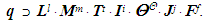(6)

3. l, m... f are exponents of the variables, the range of each has a maximum and minimum value; according to [20], integers are the following:

(7)

4. The exponents of variables can only take integer values [20], so the number of choices of dimensions for each variable, according to (7), is the following:

(8)

5. The total number of dimension options of physical variables equals

(9)

where "-1" corresponds to the case where all exponents of the primary variables in the formula (6) are treated to zero dimension.

6. According to the axiom c, the value includes both required, and inverse variables (for example, L¹ – length, L^-1 – running length). The object can be judged knowing only one of its symmetrical parts, while others structurally duplicating this part may be regarded as information empty. Therefore, the number of options of dimensions may be reduced by ω = 2 times. This means that the total number of dimension options of physical variables without inverse variables equals .

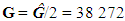7. For further discussion we use the methods of the theory of similarity, which is expedient for several reasons. In the study of the phenomena occurring in the world around us, it is advisable to consider not individual variables but their combination or complexes which have a definite physical meaning. Methods of the theory of similarity based on the analysis of integral-differential equations and boundary conditions, allow for the identification of these complexes. In addition, the transition from DL physical quantities to dimensionless (DS) variables reduces the number of variables taken into account. The predetermined value of DS complex can be obtained by various combinations of DL variables included in the complex. This means that when considering the challenges of new variables we take into account not an isolated case, but a series of different events, united by some common properties. It is important to note that the universality of similarity transformations is defined by the invariant relationships that characterize the structure of all the laws of nature, including for the laws of relativistic nuclear physics. Moreover, dimensional analysis from the point of view of the mathematical apparatus has a group structure, and conversion factors (the similarity complexes) are invariants of the groups. The concept of the group is a mathematical representation of the concept of symmetry, which is one of the most fundamental concepts of modern physics [21].

According to π-theorem [22], the number of possible DS complexes (criteria) with ξ = 7 main DL variables for SI will be

(10)

Applying the theory of similarity is motivated by the desire to generalize obtained results in the future for different areas of physical applications. The numerical value of can only increase with the deepening of knowledge about the material world. It should be mentioned that the set of DS variables is a fictitious system, since it does not exist in physical reality. However, this observation is true for proper SI too. At the same time, the object which exists in actuality may be expressed by this set.

The relationships (6)–(9) are obtained on the basis of the principles of the theory of groups as set forth in [17]. The present results provide a possible use of information theory to different physical and engineering areas with a view to formulating precise mathematical relationships to assess the minimum comparative uncertainty (see section 3.2) of the model that describes the studied physical phenomenon or process.

3.2. Information Quantity Inherent to Model

The validity of a mathematical model structure is confirmed, to a researcher, by the small differences between theoretical calculations and the experimental data. In doing so a question is overlooked: to what extent does the chosen model correctly describe the relevant natural phenomenon or process.

In [23] it has been shown that by setting a priori the total value of uncertainties of an experiment and the formulated model, one can determine the necessary number of measurements of the chosen variable and the validity of the selected model. The specified approach at the decision of inverse mathematical tasks is based on the legitimacy of a condition [24]:

(11)

where y is the set of characteristics of the investigated process; v is an experimental field of measurement; G denotes the set of possible theoretical fields of measurements g; B is the law connecting the characteristic of investigated object y with g; ρ_G (g₁, g₂) is a measure of affinity ("distance") between two fields; and Δ is an absolute uncertainty of definition of a field g.

The condition (11) means that the field, calculated under the characteristic y, is from v on distance, smaller or equal Δ. In what follows, we denote Δ_pmm as the uncertainty in determining the DS theoretical field u, "embedded" in a physical-mathematical model and caused only by its dimension that is the property of the model to reflect a certain number of characteristics of researched phenomena, its external and internal connections. What is the possible structure of Δ_pmm? To answer this question, we turn to [25], in which there has been reviewed some attempts to find a more general measure of information than the Shannon concept. In addition, the need for such an alternative measure has been demonstrated based on a historical review of the problems concerned with the conceptualization of information. The author has proven that an alternative measure can be presented in the context of a modified definition of information applicable outside of the conduit metaphor of Shannon’s approach. There has been shown several features superior to those of entropy. For instance, unlike entropy it can be easily and consistently extended to continuous probability distributions, and unlike differential entropy this extension is always positive and invariant with respect to linear transformations of the coordinates. The author has proven a theorem, which is interpreted as an assertion that the total information amount can be separated into information identifying the element of the partition, plus the average information identifying an element within subsets of the partition. Taking into account this conclusion, we can represent Δ_pmm as the sum of two terms, in which a first term of an alternative measure of information defines Δ_pmm' and the second term dictates the choice of Δ_pmm''

(12)

where Δ_pmm' is the uncertainty due to COP, which is associated with the reduction in the number of recorded primary variables compared with SPV; and Δ_pmm'' is the uncertainty due to the choice of the number of recorded influencing variables within the framework of the set of COP.

The equation (12) is an expression of the fact that during modeling of any phenomenon or technological process and equipment there is a gap between the researched object and its theoretical representation in physical-mathematical form due to choosing only COP and a number of variables recorded by the conscious observer due to their knowledge, experience and intuition. The reality of the environment is the obvious a priori condition for the modeling of the investigated material object. By allocating the interested process or phenomenon, the unknown relationships between the content of object and the environment are "broken". In this context it is obvious that an overall uncertainty of the model including inaccurate input data, physical assumptions, the approximate solution of the integral-differential equations, etc., will be larger than Δ_pmm. Thus, Δ_pmm is only one component of a possible mismatch of real object and its modeling results. In turn, Δ_pmm'' cannot be defined without declaration of the chosen COP (Δ_pmm'). So, according to its nature, Δ_pmm will be equal to the sum of two terms. When comparing different models (according to a value of Δ_pmm) describing the same object, preference should be given to the model for which Δ_pmm/Δ_exp is closer to 1. The uncertainty Δ_exp is the estimated uncertainty in the determination of the generalized objective function (similarity criterion) during an experiment or computer simulation. It will be always larger than Δ_pmm. Many different models may describe essentially the same object, where two models are considered to be essentially the same if they are indistinguishable from a value of Δ_pmm.

We formulate an approach for the introduction of a measure of the information quantity about an object in SPV and the definition of a sequence of actions (algorithm) allowing a measurement of this quantity. A certain complexity of the observed material object is offered as a measure of the complexity of the object model. Each observer can decide only the category of the model. Any claim can be made only with respect to the model. Of course, the notion of "complexity" also requires definition, and there is a possibility of arbitrariness. However, the process of cognition of a real object as a physical system, in general, is infinite. Thus, the model of the system is a formal structure built according to certain rules, and the design certainly is predictable. In this case, a material object (a certain totality) can be represented in two different ways. By merely listing its elements when the researcher supposes that a set of values is finite, or by specifying a system of rules (algorithm), based on which you can perform such an enumeration. This means a totality is thus accounted for. From a practical point of view, the most natural assertion is that the measure of complexity of the totality is the number of elements contained therein. So, one of the simplest ways is to find the magnitude calculated according to the number of elements included in this description. This value is an information quantity measure contained in the description of a physical system. In order to calculate an information quantity we choose Х₁, Х₂,.... Х_n (n Є N) primary variables. Then [17] for a secondary variable, primary variables enter into the formula of dimension with exponents τ₁, τ₂, ..., τ_n Є P, where Р is the set of rational numbers. If the set of values Ε_τn, which can accept τ_n in various variants of formulas of dimension for secondary variables, has the top and bottom verges, then Ε_τn is finite [26]. Consideration of a case τ_nЄ R, τ_nЄ Ε_τn, Ε_τnЄ R, where R is a totality of real numbers, is invalid as then it is possible τ_nЄ R\Р, where τ_n represents an irrational number does not have physical meaning. The number of elements in Ε_τn will make е_n. The variant dimension number of physical variables describing the internal structure of a material object reaches Ğ = Πе_n – 1, where "-1" corresponds to the occasion when all exponents of primary variables in the formula are treated to zero dimension.

As the information quantity of an object is connected to its symmetry [27], the number Ğ can be reduced by a factor of ω (quantity of equivalent parts in the researched material object): G = Ğ / ω. Obviously, the equivalent parts of a symmetrical object {Ε_τn} have identical structure, where {Ε_τn} is the totality including elements of Ε_τn totalities. Consequently, the object can be judged, knowing only one of its symmetrical parts, while others structurally duplicating this part, may be regarded as information empty. Knowing G and using π-theorem [22], as it is mentioned in Chapter 3.1, the number of DS complexes א_SI equals to the number of DL physical parameters G, net amount of ξ primary parameters, i.е. א_SI = G – ξ. For further discussion we will assume that each DS complex represents the original readout through which some information on DS researched field u can be obtained [28]. It is supposed that the accounting of readouts (complexes) is equiprobable. Use of the concept "readout" in examining some object at the stage of the model development is due to the expediency of the vector (positional) ways of representing information of the observed phenomena. When there are a large numbers of components (a large-dimensional vector space) it is possible to distinguish only two states of the vector component: for example, presence or absence of a signal, in our case the appearance or lack of a readout-variable [29]. It should be noted that the approval of the equiprobable occurrence of a readout is justified by the purpose of the research – finding the absolute uncertainty Δ_pmm stipulated by the level of the detail of the researched object. Indeed, any other distribution of readouts yields less information [25, 30], which leads to a larger uncertainty in comparison with an uncertainty calculated at the uniform distribution of readouts.

This approach completely ignores the human evaluation of information. In other words, a set of 100 notes played by chimpanzees, and a melody of Mozart’s 100 notes in his Piano Concerto No.21-Andante movement, have exactly the same amount of information. Let there be א_SI readouts, such that there is an uncertainty directly related to א_SI. That is, the larger the א_SI, the greater the uncertainty. Its measured numerical value is called entropy, and may be calculated by the formula [28]:

(13)

where k is Boltzmann's constant.

When a researcher chooses the influencing factors (the conscious limitation of the number of variables describing an object), the mathematical model entropy is decreased a priori. It is natural to measure the entropy change by a parameter [30]:

(14)

where ΔH is entropy difference between the two cases, pr – "a priori", ps - "a posterior".

If one considers that the efficiency Q [28] of the passive mental method as equal to one because just a thought experiment is conducted and no distortion is brought into the real system (modeler is thinking only), then one can write according to (14):

(15)

where ΔA is the a priori information quantity about the material object.

Using Equations (13), (14), (15) and imposing symbols: z' being the number of physical DL values in the selected COP (see 3.1), β' is the number of primary physical DL values in the selected COP, we obtain:

(16)

where ΔA' is the a priori amount of information quantity about the observed object due to the choice of COP.

The value ΔA' is linked to Δ_pmm' and S (the DS interval of supervision of a field u) by the dependence [28]:

(17)

Substituting (15) into (16):

(18)

Following the same reasoning, it can be shown that Δ" is the following:

(19)

where z" is the number of physical DL variables recorded in a mathematical model; β" is the number of primary physical DL variables recorded in a model. Then, summarizing Δ_pmm' and Δ_pmm'', one can estimate the value Δ_pmm.

All of the above could be summarized as follows in the form of א –hypothesis: Let during a model formulation the chosen system of primary variables with the total number of DL physical variables be denoted by G, ξ of which are of independent dimension. In the framework of the class of phenomena (the total number of DL variables (z'), the number of primary DL variables (β') there is a dimensionless field u raised in a given range of values S. Then the absolute uncertainty of u calculation (for a given number of recorded physical DL variables z", of which β" is the number of recorded primary physical DL variables) can be determined from the relationship:

(20)

where ε = Δ_pmm/S is the comparative uncertainty [28].

Using formula (20), one can find the recommended uncertainty value with the theoretical analysis of the physical phenomena. Moreover, equation (20) also can inform a limit on the advisability of obtaining an increase of the measurement accuracy in conducting pilot studies or computer simulation. It is not a purely mathematical abstraction. Equation (20) has physical meaning. This relationship testifies that in nature there is a fundamental limit to the accuracy of measuring any observed material object, which cannot be surpassed by any improvement of instruments and methods of measurement. The value of this limit is much more than the Heisenberg uncertainty relation provides and places severe restrictions on the micro-physics.

At its core, Δ_pmm is an a priori conceptual "first-born" uncertainty that is inherent to any physical-mathematical model and is independent from the measurement process. The uncertainty determined by the proposed principle is not the result of measurement, it represents an intrinsic property of the model, and it is caused only by the number of selected variables and the chosen COP. Therefore, the overall uncertainty model including additional uncertainties associated with the structure of the model and its subsequent computerization will be much greater than Δ_pmm. Actually, equation (20) can be regarded as the uncertainty principle for the model development process. Namely, any change in the level of the detailed description of the observed object (z''-β''; z'-β') causes a change in the uncertainty model Δ_pmm and the accuracy of each main variable characterizing the properties of the object internal structure.

It is interesting to speculate on further applications of equation (20) for micro- and macro-physics, such as the Heisenberg uncertainty relation, the accuracy of the fine structure constant, and as applied to heat and mass transfer processes which are discussed below.

4. Applications of א -Hypothesis

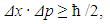
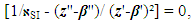
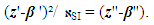
4.1. Heisenberg’s Uncertainty Relation

The numerical value of א_SI can be calculated by the use of a heuristic approach with a relative uncertainty of 410^-6, as

(21)

where α is the fine structure constant, α ^-1 = 137.035999 [31].

We apply א_SI formula (21) in order to select a modified form of Heisenberg's uncertainty relation for one dimensional space [32]. The theoretical limit of accuracy of any measurements for the DL standard deviation of coordinates Δx (uncertainty of position) and DL standard deviation of the momentum Δp (uncertainty of momentum) is the following

(22)

where ħ = h/(2π), and h denotes Planck's constant.

We take into account that comparative uncertainties of DL researched variable x and DS researched variable X which are equal to:

(23)

or

(24)

where S_x* is the DL considered range of changes of the measured DL variable x, S_x denotes the DS considered range of changes of the measured DS variable X, r* denotes the DL scale parameter with the same dimension that x and S_x* have, and ΔX denotes the DS standard deviation of coordinate X.

We can obtain:

(25)

(26)

where ΔP denotes the DS uncertainty of the DS momentum P, S_p denotes the DS considered range of changes of the DS momentum P.

Due to analyzing of recorded variables dimensions, the model of Heisenberg's uncertainty relation is classified with COP_SI ≡ LMT. In order to formulate the conditions for achieving the minimum comparative uncertainty of a model (ε_min)_LMT, it is required to equate its partial derivative with respect to z'- β', to zero. Thus we can obtain:

(27)

(28)

(29)

So, (ε_min)_LMT can be reached at the following data:

(30)

(31)

where "-1" corresponds to the case when all the primary variable exponents are zero in formula (6); dividing by 2 indicates that there are direct and inverse variables, e.g., L¹-length, L^-1- run length, and 3 corresponds to the three primary variables L,M,T.

And (ε_min)_LMT equals

(32)

(33)

where (ε_xmin)_LMT and (ε_pmin)_LMT are minimum comparative uncertainties, respectively, of DS variables X and P.

Then

(34)

(35)

Taking into account (22), (24), (34) and (35),

(36)

where S_p* is the DL considered range of changes of the measured DL variable p.

Then the modified Heisenberg's uncertainty relation can be introduced with a relative uncertainty of 910^-6 in the following form

(37)

where γ is Euler's constant, 0.577216; β=1/1,836.152746, β = m_e/m_p, m_e is the electron mass, 9.10938310^-31 kg, and m_p is the proton mass, 1.67262210^-27 kg [20].

The modified theoretical limit of accuracy of any measurements connects the DL considered range of changes of the measured DL variable x and the DL considered range of changes of the measured DL variable p. According to the aforementioned investigation the expression S_x*· S_p* (37) can be regarded as a first approximation, as a real constant in space and time because its value depends essentially on α, e, γ, β and ħ.

This equation (37) is objective and independent from the presence of the conscious observer conducting measurements. Thus, according to equation (36) the interval of the particle location and the interval of the particle momentum cannot be known with absolute precision simultaneously. The more precisely one specifies the location of the particle, the larger the degree of uncertainty of the particle's momentum, and vice versa.

Equation (37) is in fact a possible interpretation of a general principle of W. Heisenberg (22) in another form, which holds for any investigated object. At the same time, it is understood that without enough comparison with previous results, the readers cannot evaluate whether the introduced results are good or bad. That is why further examples, maybe, can convince researchers for the appropriateness of the א –hypothesis for experiments in engineering and physics.

4.2. Heat and Mass-Transfer

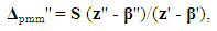
The process of heat transfer by freezing a thin layer of paste material posted onto a moving cooled cylinder wall has been investigated [33]. According to analysis of the recorded variables dimensions, the model is classified by COP_SI ≡ LMTΘ.

Let’s calculate z'-β'. According to (8)

(38)

where "-1" corresponds to the case where all the primary variables exponents are zero in formula (6); division by 2 indicates that there are direct and inverse variables, e.g., L¹-length, L^-1- run length; and 4 corresponds to four primary variables L,M,T,Θ .

The minimum comparative uncertainty of a model (ε_min)_LMTθ, can be reached at condition (29). Then we obtain:

(39)

Substituting (38) and (39) into (20) we find

(40)

There were recorded 18 (z*) input DL variables and 5 (β*) primary physical variables, such that we obtain z*-β*=18-5=13 for the DS criteria.

A study of the developed model by computer simulation using the random balance method has been conducted. As the objective function, the final DS temperature of the outer surface of the material was selected, where are the DL temperatures of the freezing point of a material, outer surface of a material layer and evaporation point of the refrigerant, respectively. are the DL uncertainties of measurement of these temperatures. Their declared values were:

The declared achieved discrepancy between the experimental and computational data in the range of admissible values of the similarity criteria and dimensionless conversion factors did not exceed 8%.

Taken into account was the fact that the direct measurement uncertainties are much smaller than the measured values, accounting for a few percent or less of them. The uncertainty can be considered formally as small increments of a measured variable. In practice, finite differences are used, rather than the differentials. So, in order to find the value of an absolute DS uncertainty , the mathematical apparatus of differential calculus was applied [34]:

(41)

where denotes the partial derivatives of the function with respect to one of the several variables that affect ; and denotes the uncertainty of the variable .

For the present example, according to equation (40), one can find an absolute total DS uncertainty of the indirect measurement , reached in the experiment:

(42)

From equation (20), using calculated values (9), z'-β' (38), and (z''-β'') (39), one obtains a DS uncertainty value of the chosen model:

(43)

where is the DS given range of changes of the DS final temperature allowed by the chosen model [33].

From (42) and (43) we get , i.e., an actual uncertainty in the experiment is 1.7 times (0.066/0.038) larger than the possible minimum. It means, at the recorded number of DS criteria the existing accuracy of the DL variable’s measurement is insufficient. In addition, the number of the chosen DS variables z*-β* = 13 is less than the recommended ≈ 19 (39) that corresponds to the lowest comparative uncertainty at COP_SI ≡ LMTΘ. That is why, for further experimental work it is required to use devices of a higher class of accuracy sufficient to confirm/clarify a new model designed with many DS variables.

In this example we introduce a full explanation of the required steps for analyzing experimental data and compare it with results obtained from a field test or computer simulation of model.

4.3. The Fine Structure Constant

4.3.1. First Example

In [31] the authors have reported a new experimental scheme which combines atom interferometry with Bloch oscillations leading to a new determination of the fine structure constant (FSC) = 137.03599945(62) with a relative uncertainty r₁ of . In this case the absolute uncertainty was . The declared range S₁ of variations was . Research is organized into the frame of COP_SI ≡ LMТ.

One can calculate the achieved comparative uncertainty as

(44)

For the mechanical processes (COP_SI ≡ LMТ), taking into account (8), (10) and (29), the lowest comparative uncertainty (Δ_pmm/S)_LMT that can be reached occurs under the following conditions:

(45)

(46)

where "-1" corresponds to the case when all the primary variables exponents are zero in formula (6); division by 2 indicates that there are direct and inverse variables, e.g., L¹-length, - run length; and 3 corresponds to three primary variables L,M,T.

We obtain:

(47)

The calculated comparative uncertainty ε₁ = 0.4503 is much higher than that recommended (see equation (47)) according to the discussed approach. So, the above-mentioned method and apparatus should measure the FSC value with a greater accuracy.

4.3.2. Second Example

A recoil-velocity measurement of Rubidium has been conducted and a new determination of the FSC as = 137.035999037(91) with a relative uncertainty of [35]. In this case the absolute uncertainty was . The description of the experimental unit and methods corresponded to COP_SI ≡ LMТ. According to equation (47), the lowest comparative uncertainty is equal to 0.0048. The range of variation S₂ of is . In this case, the comparative uncertainty of the experimental method is

(48)

This value is larger than the lowest comparative uncertainty for COP_SI ≡ LMТ calculated according to equation (47). For this reason the research team knows the limiting value of achievable accuracy and can try to find different strategies for obtaining optimum results.

The two studies discussed above differ from each other by the design of the experimental setups and methods of measurement. However, in the framework of the suggested approach it can be argued that a greater accuracy in the measurement of FSC was achieved in [35].

4.3.3. Third Example

Analysis of the FSC measurements made during 2006-2014. None of the current experimental measurements which calculate the FSC have declared an uncertainty interval in which the true value can be placed. Therefore, in order to apply the stated approach, as an estimated e error interval of FSC, we choose the difference of its value reached by the experimental results of two projects: (α') ^-1 = 137.035999872 [36] and (α'') ^-1 = 137.035999038 [35]. In this case the possible observed range S* of (α) ^-1 variation is equal to

(49)

Following the same scheme of reasoning that was introduced in Chapters 4.3.1 and 4.3.2, and taking into account (47), we analyzed several scientific original publications and CODATA (Committee on Data for Science and Technology) recommendations over the past nine years from the perspective of the achieved comparative uncertainty value. The data are summarized in Table 1 and Figure 1.

Table 1. Results of the fine structure constant measurements during 2006-2014 including the achieved comparative uncertainty

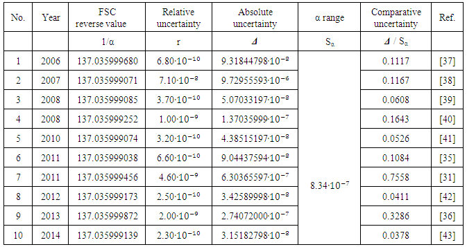
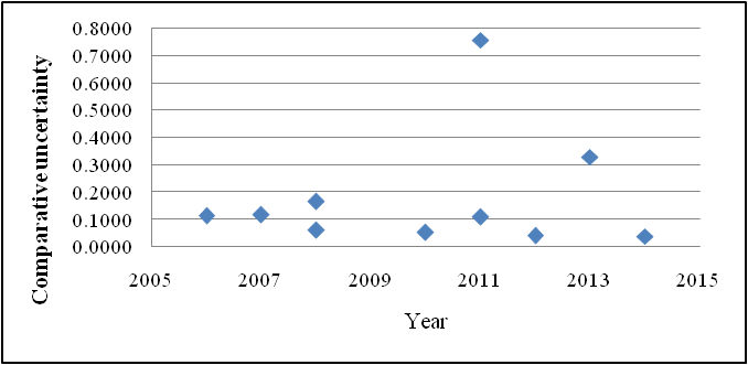Figure 1. A graph summarizing the partial history of the fine structure constant measurement displaying the decrease of the comparative uncertainty

As a rule, when considering the accuracy of the achieved results during the FSC measurement the concept of relative uncertainty is used. However, this method for identifying the measurement accuracy does not indicate the direction in which one can find the true value of FSC. In addition, it involves an element of subjective judgment [44]. For this reason we use the comparative uncertainty.

It can be seen from the data given in Table 1 and Figure 1 that the affirmations presented in [40] are only partially confirmed. The fact is that there has been a dramatic improvement in the accuracy of measurement of the FSC during last decade. This is verified by using the calculated value of the relative uncertainty, the smallest achievable value of which has not been mentioned. However, judging the data by the comparative uncertainty according to the proposed approach, one can see that the measurement accuracy has not significantly changed. Perhaps this situation has arisen as a result of unaccounted systematic errors in these experiments. At the same time, it must be noted that in all likelihood, the exactness of the FSC measurements, as other fundamental physical constants, cannot be perfect. Therefore the development of a larger number of designs and improvements of various experimental facilities for the measurement of the FSC is required in order to bring results closer to the minimum comparative error (ε_min)_LMT.

We can argue about the order of the desired value of the relative uncertainty (r_min)_LMT . For this purpose we take into account the following variables: (47), (49). Then the lowest possible absolute uncertainty for COP_SI ≡LMТ is equal to

(50)

In this case the lowest possible relative uncertainty (r_min)_LMT for COP_SI ≡LMТ is the following:

(51)

This value corresponds to recommendations mentioned in [45] and should satisfy the existing standards community.

5. Discussion

Despite the apparent attractiveness and versatility of the suggested approach, there are certain limitations, restrictions and occasions where its applicability is limited. They include the following:

- The information-based approach requires the probable appearance of variables chosen by a conscious observer. It ignores factors such as developer knowledge, intuition, experience and environmental properties;

- The approach requires the knowledge or declaration of the uncertainty interval of the main observed or researched variable. In reality, the value of this parameter is not declared in any serious experimental research in physics and engineering. Sometimes the uncertainty interval, for example, of Planck's constant, the speed of light and other fundamental physical constants, is mentioned in the review articles only in order to confirm the convergence of the experimental data to a certain value or reducing the spread of the results;

- The method does not give any recommendations on the selection of specific physical variables, but only places a limit on their number.

Nevertheless, the approach yields the universal metric by which the model discrepancy can be calculated. A more effective solution to finding the minimum uncertainty can be reached using the principles of information and similarity theories. Qualitative and quantitative conclusions drawn from the obtained relations are consistent with practice. They are as follows:

Based on the information and similarity theories, a theoretical lowest value of the mathematical model uncertainty of the phenomenon or technological process can be derived. A numerical evaluation of this relation requires the knowledge of the error interval of the main researched variable and the required number of variables taken into account. In order to estimate the discrepancy between the chosen model measurement and the observed material object, a universal metric called comparative uncertainty has been developed further. Our analytical result for ε = Δ_pmm/S is a surprisingly simple relation.

The author has carried out a theoretical evaluation of Heisenberg's uncertainty relation based on a mathematical formulation of the comparative uncertainty. This is the first time that this has been examined. When analyzing the modified Heisenberg uncertainty relation, the error interval of the particle location and the error interval of the particle momentum cannot be known with absolute precision simultaneously. This is an objective fact and is independent of the presence of the conscious observer conducting measurements. The more precisely the location of the particle is specified, the more uncertain a measurement of the momentum will be, and vice versa.

Many attempts have been made to optimize a mathematical model of technological process or equipment which could bypass this. At that time, information and similarity theories were available for this purpose only. Satisfactory solutions could be achieved by applying the א-hypothesis and by taking the optimum number of variables into account. In addressing applications such as heat and mass transfer, full explanations of the required steps for analyzing experimental data and comparison with results obtained by a field test or computer simulation are introduced. From the present investigation one can conclude that the fundamentally novel analysis determines the most simple and reliable way to select a model with the optimal number of selected variables. This will greatly diminish the duration of the studies as well as the design stage, thereby reducing the cost of the project.

The proposed methodology is an initial attempt to use a comparative uncertainty instead of relative uncertainty in order to compare the measurements results of the FSC and to verify its true value. A direct way to obtain reliable results has always been open, namely to assume that the FSC value lies within a chosen interval. However, this idea cannot be proved because of the difficulty of specifying the possible limit of the relative uncertainty. Of course, the choice of a value of the variation of (α) ^-1, S*, is controversial because of its apparent subjectivity. With these methods, our capacity to predict the FSC value by usage of the comparative uncertainty allows for an improvement of our fundamental comprehension of complex phenomenon, as well as allowing us to apply this understanding to the solution of specific problems. It may be the case that such findings will induce a negative reaction on the part of scientific community and some readers who consider the above examples as a game of numbers. In his defense, the author notes that eminent scientists such as Arnold Sommerfeld, Wolfgang Pauli and others scientists have followed a similar approach in order to approximate values for the FSC. The calculated results are routine calculations from formulas known in the scientific literature. At the same time, an additional perspective of the existing problem will, most likely, help us to understand the existing situation and identify concrete ways for its solution. Reducing the value of the comparative uncertainty of the FSC to the lowest achievable value of 0.0048 for the chosen COP_SI ≡LMТ will serve as a convincing argument for professionals involved in the perfecting of SI.

6. Conclusions

The measurement theory and its concepts remain a precise science today, in the twenty-first century, and will continue to be the case forever (a paraphrase of Prof. Okun [46]). The use of the א-hypothesis only limits the domain of applicability of measurement theory for uncertainties that are much larger than the uncertainty of the physical-mathematical model due to its finiteness.

א-hypothesis might be applicable to experimental verification. In general, it is available when the researcher has all the information about the uncertainty interval of the main variable.

The quantification of the model uncertainty via the information quantity value embedded in the physical-mathematical model opens up the possibility of linking the experimental and theoretical investigations by adopting the proposed approach for investigations into various physical phenomena or technological processes.

The comparative uncertainty concept for calculating the optimal number of recorded variables and derived effects which are amenable to rigorous experimental verification have been introduced.

One of the main results in the present paper is the proof of a necessary and sufficient condition for the correct choice of the number of variables recorded in a mathematical model describing physically observed phenomena and measurement processes.

The author has proposed that the estimate of the a priori achievable uncertainty of a mathematical model due to a model’s finiteness (limited number of chosen variables), can be a peculiar metric for the assessing the accuracy of experimental measurements and computer simulation data.

The author also hopes this paper stimulates readers to participate in the development of this approach in different fields of physics and engineering.