N. M. Yagmurlu, B. Karaagac, S. Kutluay
Department of Mathematics, Inonu University, Malatya, Turkey
Copyright © 2017 Scientific & Academic Publishing. All Rights Reserved.
This work is licensed under the Creative Commons Attribution International License (CC BY).
http://creativecommons.org/licenses/by/4.0/

Abstract
In this study, numerical solutions of Rosenau-RLW equation which is one of Rosenau type equations have been obtained by using Galerkin cubic B-spline finite element method. The fourth order Runge-Kutta technique has been used to solve the resulting ordinary differential equation system occured by the application of the method. The accuracy and efficiency of the present method have been tested by calculating the error norms  and
and  Moreover, the computed results have been compared with exact and numerical ones existing in the literature.
Keywords:
Finite element method, Rosenau-RLW equation, Galerkin method, Runge-Kutta, Cubic B-spline, Solitary wave, Interaction
Cite this paper: N. M. Yagmurlu, B. Karaagac, S. Kutluay, Numerical Solutions of Rosenau-RLW Equation Using Galerkin Cubic B-Spline Finite Element Method, American Journal of Computational and Applied Mathematics , Vol. 7 No. 1, 2017, pp. 1-10. doi: 10.5923/j.ajcam.20170701.01.
1. Introduction
Nonlinear evolution equations play an important role for the studies appeared in nonlinear sciences. These equations can be seen in many studies on nonlinear evolutions such as plasma physics, solid state physics, fluid mechanics, water wave mechanics, meteorology and nonlinear optics. Two important equations belonging to the class of nonlinear evolution equations are  | (1) |
 | (2) |
namely KdV and RLW equations, respectively. While KdV equation (1) is a nonlinear model to study the change forms long waves advancing in a rectangular channel, RLW equation (2) is used to simulate wave motion in media with nonlinear wave steeping and dispersion, such as shallow water waves and ion acoustic plasma waves. From the studies on KdV equation, it is well known that the KdV equation has a number of shortcomings. Firstly, it describes an unidirectional propagation of waves. Thus wave-wave and wave-wall interactions can not be treated by the KdV equation. Secondly, both shape and the behavior of high-amplitude waves can not be well predicted by the KdV equation since it was derived under the assumption of weak an harmonicity. In order to overcome these shortcomings of KdV equation, Rosenau [1, 2] has introduced an equation in the form  | (3) |
which is called Rosenau equation. The existence and uniquness of Rosenau equation (3) was proved by Park [3]. Later on, to make more advanced studies on nonlinear waves and to understand other nonlinear behaviours of the waves, the term  was added to Rosenau equation (3) and the following form has been obtained
 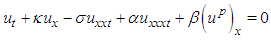 | (4) |
where  are real constants and
  is an integer. This equation is called as generalized Rosenau-RLW equation [4]. There are miscellaneous studies about Rosenau-RLW equation. For example; Zuo et. al [5] have proposed a new conservative difference scheme and also proved the corresponding convergence of the scheme. Pan et. al [6] have studied the initial-boundary problem of the usual Rosenau-RLW equation by finite difference method designing a conservative numerical scheme preserving the original conservative properties for the equation. In Ref. [7], Mittal and Jain have applied B-spline collocation method to the generalized Rosenau-RLW equation to obtain the numerical solutions with the aid of quintic B-spline base functions. Pan et al. [8] have considered the numerical solutions of the Rosenau-RLW equation using Crank-Nicolson type finite difference method and derived the existence of numerical solutions by Brouwer fixed point theorem. Hu and Wang [9] have studied the initial-boundary value problem for Rosenau-RLW equation by proposing a three-level linear finite difference scheme and also obtained the existence, uniqueness of difference solution, and a priori estimates in infinite norm. In Ref. [10], Wongsaijai and Poochinapan have proposed a mathematical model to obtain the solution of the nonlinear wave by coupling the Rosenau-KdV and the Rosenau-RLW equation. Wang et al. [11] have designed new conservative nonlinear fourth-order compact finite difference scheme for Rosenau-RLW equation given together with initial and boundary conditions. Cai et al [4] have considered Rosenau type equations, namely Rosenau-KdV and Rosenau-RLW equations and constructed the variational discretization for solving the evolutions of solitary solutions of this class of equations. In the present study, the Rosenau-RLW equation (4) for
  is going to be considered with the following initial and boundary conditions
 | (5) |
 | (6) |
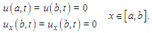
where  is sufficiently differentiable function,
  denotes the partial derivative with respect to space. The rest of the study can be summarized briefly as follows: In the second section, Galerkin finite element method has been applied to Rosenau-RLW equation. For both the element shape functions and weight functions are taken as cubic B-spline base functions. The system of equations obtained in terms of element parameters has been solved using the fourth-order Runge-Kutta technique. In the third section, two numerical problems, namely movement of solitary wave and the interaction of two solitary waves, are studied for the problem with initial and boundary conditions. The obtained numerical results are presented both in tabular and graphical format. Moreover, the computed results are also compared with some of those available in the literature.
2. Galerkin Finite Element Model for Rosenau-RLW Equation
Finite element method is one of the numerical methods used to obtain approximate solutions of ordinary and partial differential equations. In this study, Rosenau-RLW equation (4) for  is considered with the initial and boundary conditions (5) and (6), respectively. We will to obtain the numerical solutions of the problem with the aid of Galerkin finite element method. For this purpose, first of all, the solution domain of the problem
  is divided into
  finite elements with the nodal points denoted by
  as
as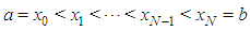 When each term in Rosenau-RLW equation (4) is multiplied by the weight function
  and integrated by parts over the region, we obtain the weak form of Rosenau-RLW equation is obtained as
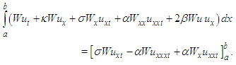 Therefore, the weak form for a typical element on
  is given as
 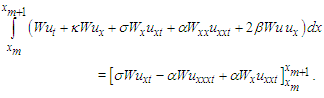 | (7) |
In order to construct the approximate solution  corresponding to the exact solution
  of the problem and to derive element equations the element shape functions are determined. The following cubic B-spline base functions have been choosen as element shape functions [12]
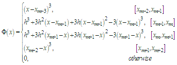 The approximate solution
  in terms of cubic B-spline bases
  and time-dependent element parameters
  on the whole region can be defined as
 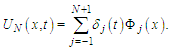 In order to define cubic B-spline base functions for a typical element on
  the local transformation
  for
for  is applied, and the following base expressions are obtained
 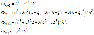 | (8) |
The approximate solution on a typical element  can be written in terms of local coordinate system as
 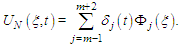 | (9) |
As it is known, in Galerkin finite element method, the weight functions  are taken as the same base functions
  used in approximate solution. If we use the weight functions and the approximate solution (9) in the weak form (7), we obtain the element equation for a typical element on
  as
as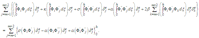 In the last equation, the integrals are represented by the following notations
 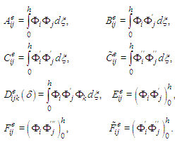 From here, after some calculations, the following element matrices are obtained
 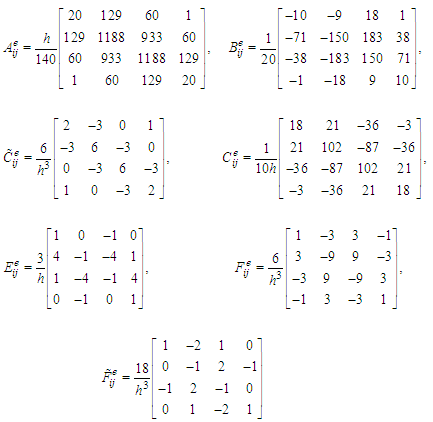 and
and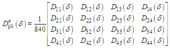 where
where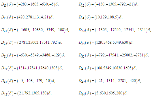 Thus, for a typical element on
  the element equation in the matrix form is obtained as
  where
where 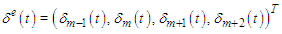 are element parameters and
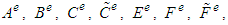
 element matrices. In order to represent the whole system, if all of the elements on the whole domain are combined then the following system of algebraic equations is obtained
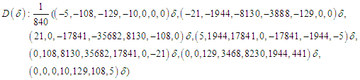
 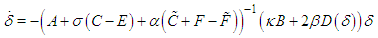 | (10) |
where 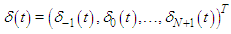 and
and 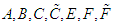 ve
ve  are defined for the whole region. The generalized th rows of the matrices can be stated as follows
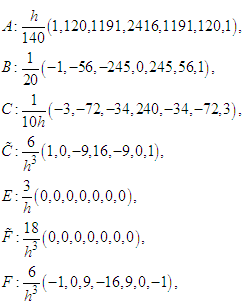
 The system of algebraic equations (10) is composed of
  unknowns and
  equations. Before starting the solution of the system, the application of the boundary conditions which is one of the important steps of the method is applied. For this process, the boundary conditions
 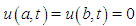 and the values of
  at nodal points
  for
for  and
and  are used
 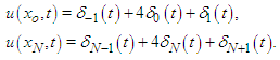 Using these equations, the parameters
  and
and  are eliminated from the system (10) with a simple algebraic manipulation. Thus, the system (10) is now reduced into a system of
  In the obtained algebraic system, the parameters
  are iteratively calculated using the parameters
  with the help of fourth-order Runge-Kutta technique. We need initial values of parameters to be able to start the Runge-Kutta technique. These initial values are taken from the initial condition of the problem
  and approximate solutions
 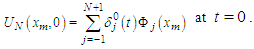 The system can be written explicitly in the form
 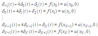 | (11) |
The system (11) is made up of  equations and
  unknowns. For this system to be solvable, two auxiliary equations are added to the system. These auxiliary equations are obtained using the boundary conditions including derivatives given by (6) at
  as
as 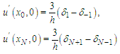 Now, the system (11) is of type
 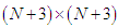 and can be stated in matrix form as
 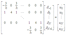 | (12) |
So, the solution of (12) results in initial parameters 
3. Numerical Examples and Results
In the previous section, Galerkin finite element method has been constructed for the Rosenau-RLW equation with the initial and boundary conditions. In this section, two numerical examples, namely the movement of solitary wave and interaction of two solitary waves have been taken into considered. In order to show the accuracy and efficiency of the method and make a comparison with other studies in the literature, the error norms defined by 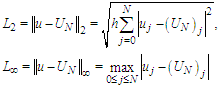 have been calculated.
3.1. Movement of Solitary Wave
Travelling of single solitary wave problem introduced by Rosenau-RLW equation has been solved for the parameters 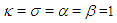 and
and  to be able to compare the results in Refs. [4-8] and Ref. [10, 11]In this study, the solution domain of the problem is taken as
  Since the exact solution of the problem is [4]
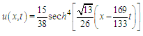 the initial condition for the problem is taken as
 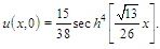 In this problem, after obtaining the numerical solutions of Rosenau-RLW equation, the error norms
  and
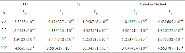
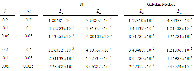
and  are calculated at various space and time steps. A comparison of the obtained error norms with some of those available in the literature has been given in tables. First of all, a comparison of the error norms on the solution domain
  for values of
  and
and  has been presented in Table 1. Then, by taking
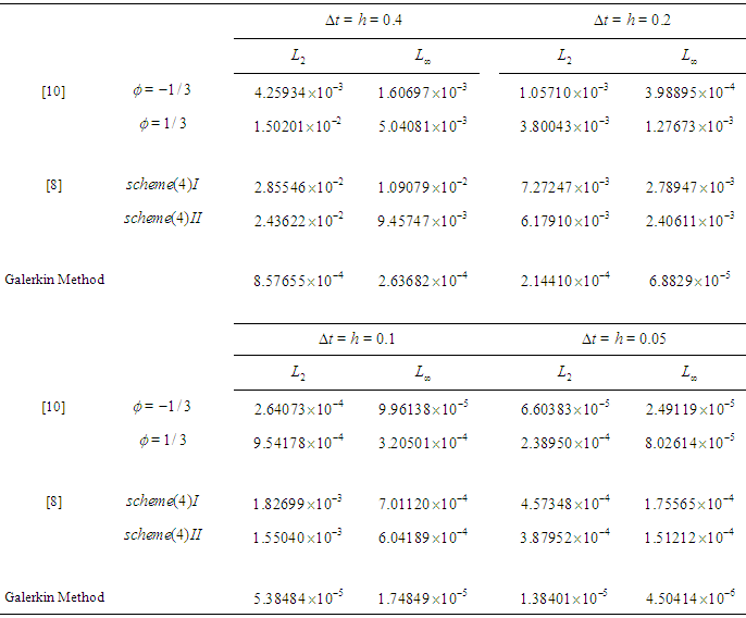
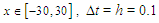
  the numerical solutions at times
  and
and  have been presented in Tables 2 and 3, respectively. Finally, in Table 4, the numerical results at various times for
  ,
,  are presented. From these tables, it is seen that when compared to other studies, the approximate solutions obtained using Galerkin finite element method are more accurate than those given in Refs. [5, 6, 8, 10, 11].
Table 1. A comparison of numerical results for
 and and

 |
| |
|
Table 2. A comparison of numerical results for
 and and

 |
| |
|
Table 3. A comparison of numerical results for
 and and

 |
| |
|
Table 4. A comparison of numerical results for
 and and

 |
| |
|
Numerical simulations of the motion of solitary wave values  and
and  are illustrated in Fig. 1. The initial amplitude of the wave at
  is
is 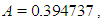 and the wave moves by almost conserving its shape and amplitude. From the numerical results, it can be seen that the solitary wave moves leaving negligible secondary waves behind it (see Fig.2).
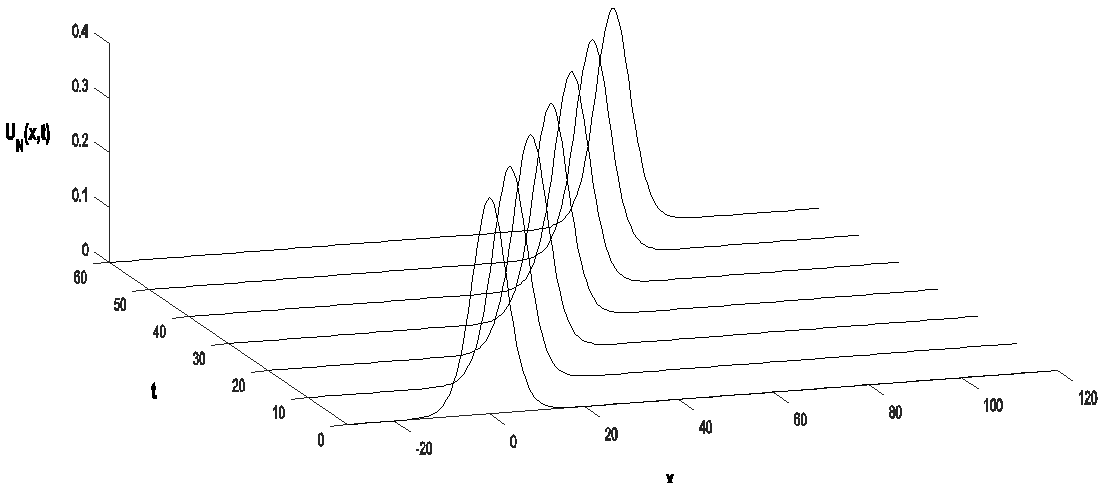 | Figure 1. The motion of a single solitary wave |
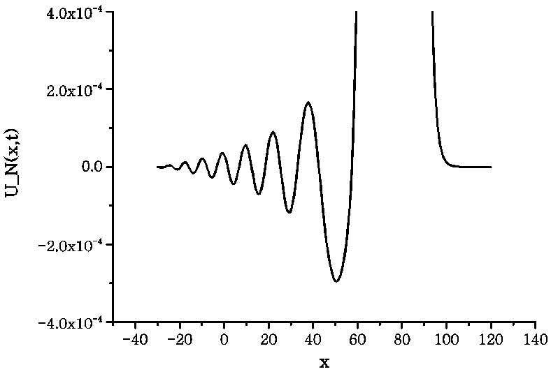 | Figure 2. Secondary waves |
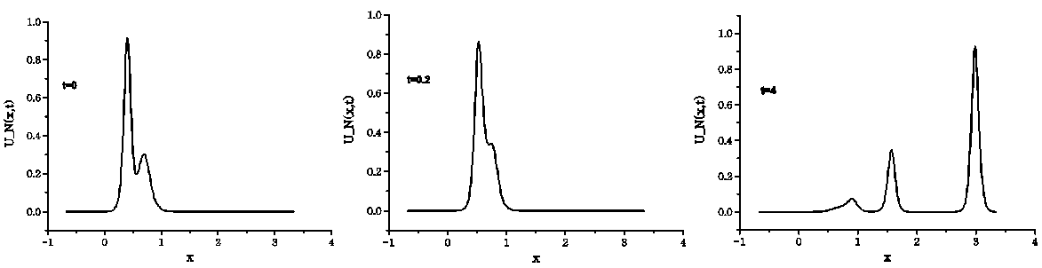
3.2. The Interaction of Two Solitary Waves
In this numerical example, the interaction of two colliding solitary waves is studied for Rosenau-RLW equation. In order to investigate the relationship between Rosenau-RLW and RLW [13-16] equations in this problem by the effect of  the parameters
  and
and  are chosen and the following initial condition is taken as
 where
where 
 The solution domain of the problem is
  , space step size is
  and time step size is
  and various values for
  are used to investigate the interaction problem [4,13]. The results for
  and
and  are obtained and numerical simulations are illustrated at times
  and 4 in Figs. 3, 4 and 5, respectively.
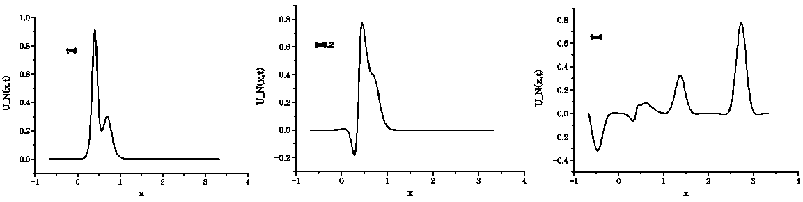 | Figure 3. The interaction of two solitary waves for 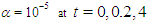 |
 | Figure 4. The interaction of two solitary waves for  |
 | Figure 5. The interaction of two solitary waves for 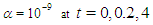 |
As it can be seen from the figure, at time  , there are two interacting waves for three values of
  . At time
  the interaction is still available and an antisoliton wave starts to appear. For small values of
  the amplitude of the antisoliton wave is smaller and for
  antisoliton is not observed. At time
  the two waves complete their interaction. Except for
  , there appears an antisoliton and several small solitons. With decreasing values of
  the amplitude of antisoliton wave decreases and the interaction problem of Rosenau-RLW equation resembles to that of RLW equation. Aditionally, similar to RLW equation, the interaction for Rosenau-RLW equation is inelastic. Secondly, to investigate the interaction for bigger values of
  we have taken
  and 8. The three dimensional graphics of the obtained results are illustrated in Fig. 6.
 | Figure 6. The interaction of two solitary waves for  and and  |
From the figures, it is seen that solitary waves do not interact, a slope is observed on the right hand side of the wave with respect to axis. It is also observed that this slope decreases by increasing values of  and solitary waves become steeper. It can be seen that the computed numerical results are also in good agreement with those in Ref. [4].
4. Conclusions
In this paper, Galerkin finite element method is successfully applied to Rosenau-RLW equation using cubic B-spline base functions. The consistency between the numerical and approximate solutions is tested by calculating the error norms  and
and  By comparing the calculated error norms with those available in the literature, it is seen that Galerkin finite element method is an useful and effective tool. It is concluded that the Galerkin finite element method can also be applied to the Rosenau type equations with other types of boundary and initial conditions to obtain their numerical solutions.
References
| [1] | P. Rosenau, “A quasi-continuous description of a nonlinear transmission line”, Physica Scripta, vol. 34, pp. 827-829, 1986. |
| [2] | P. Rosenau, “Dynamics of dense discrete systems”, Prog. Theor. Phys., vol. 79, pp. 1028-1042, 1988. |
| [3] | M. A. Park, “On the Rosenau equation in multidimensional space”, Nonlinear Anal. TMA, vol. 21, pp. 77-85, 1993. |
| [4] | W. Cai, Y. Sun, and Y. Wang, “Variational discretizations for the generalized Rosenau type equations”, Appl. Math. Comput., vol. 271, pp. 860-873, 2015. |
| [5] | J. M. Zuo, Y. M. Zhang, T. D. Zhang, and F. Chang, “A new conservative difference scheme for the general Rosenau-RLW equation”, Bound. Value Probl., vol. 2010, pp. 1-13, 2010. |
| [6] | X., Pan and L. Zhang, “On the convergence of a conservative numerical scheme for the usual Rosenau-RLW equation”, Appl. Math. Model., vol. 36, pp. 3371-3378, 2012. |
| [7] | R. C Mittal, R. K. Jain, “Numerical solution of general Rosenau-RLW equations using quintic B-splines collocation method”, Commun. Numer. Anal. 16.article ID cna-00129, pp. 1-16, 2012. |
| [8] | X. Pan, K. Zheng, and L. Zhang, “Finite difference discretization of the Rosenau-RLW equation”, Appl. Anal., vol. 92, pp. 2578-2589, 2013. |
| [9] | J. Hu and Y. Wang, “A high accuracy linear conservative difference scheme for Rosenau-RLW equation”, Math. Probl. Eng., vol. 2013, pp.1-8, 2013. |
| [10] | B. Wongsaijai and K. Poochinapan, “A three level average implicit finite difference scheme to solve equation obtained by coupling the Rosenau-KdV equation and the rosenau-RLW equation” , Appl. Math. Comput., pp. 245, pp. 289-304, 2014. |
| [11] | H. Wang, J. Wang and S. Li, “A new conservative nonlinear highg order compact finite difference scheme for the general Rosenau- RLW equation”, Bound. Value Probl., vol: 2015(77), pp. 1-16, 2015. |
| [12] | P. M. Prenter, Splines and variational methods , New York: Wiles, 1975. |
| [13] | Y. J. Sun and M. Z. Qin, “A multi-symplectic scheme for RLW equation”, J. Comput. Math., vol. 22(4), pp. 611-621, 2004. |
| [14] | A. Esen and S. Kutluay, “Application of a lumped Galerkin method to the regularized long wave equation”, Appl. Math. Comput., vol. 174(2), pp. 833-845, 2006. |
| [15] | S. Kutluay and A. Esen, “A finite difference solution of the Regularized Long-Wave equation”, Math. Probl. Eng, vol. 2006, Article ID 85743, pp. 1-14, 2006. |
| [16] | I. Dag, B. Saka and D. Irk, “Galerkin method for the numerical solution of the RLW equation using quintic B-splines”, J. Comput. Appl. Math., vol. 190, pp. 532-547, 2006. |

 Abstract
 Reference
 Full-Text PDF
 Full-text HTML