Doyo Kereyu 1, Genanew Gofe 2
1Department of Mathematics, Haramaya University, Ethiopia
2Department of Mathematics, Jimma University, Ethiopia
Correspondence to: Doyo Kereyu , Department of Mathematics, Haramaya University, Ethiopia.
| Email: |  |
Copyright © 2016 Scientific & Academic Publishing. All Rights Reserved.
This work is licensed under the Creative Commons Attribution International License (CC BY).
http://creativecommons.org/licenses/by/4.0/

Abstract
In this paper, we consider the convergence rates of the Forward Time, Centered Space (FTCS) and Backward Time, Centered Space (BTCS) schemes for solving one-dimensional, time-dependent diffusion equation with Neumann boundary condition. We present the derivation of the schemes and develop a computer program to implement it. The consistency and the stability of the schemes are described. By the support of the numerical problems convergence rates of the schemes have been determined. It is found that both methods are first order accurate in the spatial dimension in  - norm.
Keywords:
Diffusion equation, Finite difference methods, Neumann boundary conditions, Convergence rate
Cite this paper: Doyo Kereyu , Genanew Gofe , Convergence Rates of Finite Difference Schemes for the Diffusion Equation with Neumann Boundary Conditions, American Journal of Computational and Applied Mathematics , Vol. 6 No. 2, 2016, pp. 92-102. doi: 10.5923/j.ajcam.20160602.09.
1. Introduction
Consider the following one-dimensional, time-dependent diffusion equation:  | (1.1a) |
with initial condition, | (1.1b) |
and Neumann boundary conditions | (1.1c) |
 | (1.1d) |
where is an unknown function,
  and
and  are the first and second partial derivatives of the temperature
  with respect to time and space respectively,
  is the thermal diffusivity of the rod, f(x) is a prescribed initial temperature distribution over the rod, L is the length of the rod, T is a maximum time and,
  and
and  are specified functions of time t representing the heat flow across the boundaries. We assume the rod is of a homogeneous material and the surface of the rod is insulated so that heat flows only in the x-direction.This equation is also assumed to be well posed and to have a unique smooth solution u(x, t) which has sufficient regularity. The diffusion problems arise in many important applications of science and engineering, describing the distribution of temperature in a given region as a function of position and time [1, 2]. The natural conditions would be to specify the temperature everywhere in the rod at time t = 0, and use the differential equation to determine the temperature at later times by stepping along the time axis. In literature, various numerical techniques such as finite differences, finite elements and finite volumes have been developed and compared for solving one dimensional diffusion equation with Dirichlet and Neumann boundary conditions (see[1- 6]). Theoretical results have been obtained regarding the accuracy, stability and convergence of the finite difference methods (FDMs) for solving this equation. In [1, 3, 5], it is stated that for any time step size
  in the time range [0, T] and for space step size
  , FTCS method is stable if
  (r is stability limit) and BTCS method is unconditionally stable with Dirichlet boundary conditions. The authors also stated that, these methods are first-order accurate in time and second-order accurate in space. In this work, it is aimed to determine the convergence rates of the FTCS and BTCS schemes for solving equations (1.1a) - (1.1d) which are often encountered in engineering applications. The Neumann boundary condition specifies the temperature gradients across the boundaries as well as the initial temperature distribution within the rod. To solve the equation, spatial and temporal domains are discretized by the grids of points and partial derivatives occurring in the equation are replaced by approximations based on the Taylor series expansions of the function near the point or points of interest [1, 4, 5]. Since convergence is difficult to prove directly, we use an equivalent result known as the Lax Equivalence Theorem which stated that, for a given properly posed linear consistent finite difference approximation to Partial differential equation (PDE), stability is necessary and sufficient for convergence [3]. Thus, showing the consistency and stability of the finite difference scheme is sufficient for convergence. We use Gerschgorin’s Theorem to determine the stability of the methods [4], and show that FTCS method is stable if
  and BTCS method is unconditionally stable with Neumann boundary conditions. Since finite difference discretization converges at the rate of the Truncation Error (TE) (determined by the order of the spatial and temporal discretization) if the exact solution is smooth enough (see, [7]), we expand the exact solution at the mesh points of the scheme with a Taylor series and insert the Taylor expansions in the scheme to calculate the TE (difference between the resulting equation and the original PDE) and determine its order in the approximation used. Then, we see that as the discrete step sizes approach to zero, their TE also approaches to zero which indicates that the difference approximations are consistent. For the remainder of this paper, we give the details of the numerical algorithms to solve application problems involving diffusion equation. In section 2, a difference schemes for (1.1) is derived. In section 3, convergence of the schemes is described. Finally, numerical problems are given to verify the validity of the theoretical results.
2. Finite Difference Schemes
We divide x = [0, L] and t = [0, T] into M and N subintervals of equal lengths  and
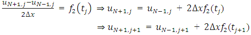
and  respectively. The Neumann boundary conditions given on equations (1.1c) and (1.1d) are approximated by the central differences. For this we introduce “ghost points”
  and
and  in addition to the grid points
  .
. 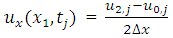 | (2.1) |
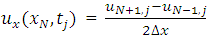 | (2.2) |
From equation (2.1) and equation (2.2), the values of  and
and  can be computed which will then be used to compute
  and
and  at the boundaries.
2.1. The Explicit (FTCS) Scheme
To form the scheme, the first derivative of the temperature with respect to time in equation (1.1a) is approximated with a forward difference and central difference is used to approximate
  about
about  , and all terms are evaluated at time j.
 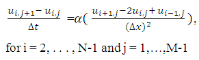 | (2.3) |
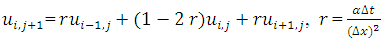 | (2.4) |
Initial condition, 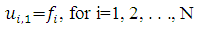 | (2.5) |
At two end points,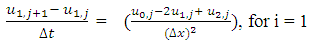 | (2.6) |
 | (2.7) |
But from equation (2.1) and equation (2.2), 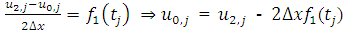 | (2.8) |
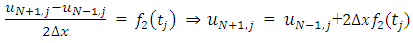 | (2.9) |
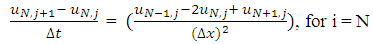
Then, by substitution equation (2.6) and equation (2.7) become; | (2.10) |
 | (2.11) |
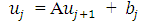
This can be written in matrix form as follows which is to be solved iteratively;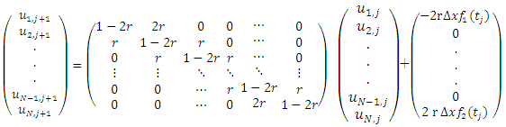 | (2.12) |
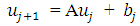 | (2.13) |
2.2. The Implicit (BTCS) Scheme
The forward time difference in equation (2.3) is replaced by the backward time difference and the space difference remaining the same to form this scheme; 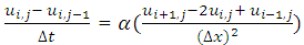 | (2.14) |
This is equivalent to;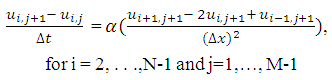 | (2.15) |
 | (2.16) |
With initial condition, 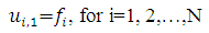 | (2.17) |
From equation (2.1) and equation (2.2), 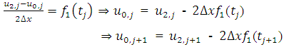 | (2.18) |
 | (2.19) |
Then, at two end points (i=1 and i=N), | (2.20) |
 | (2.21) |
This can be written in matrix form as; 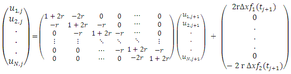 | (2.22) |
 | (2.23) |
This system of equation is a tri-diagonal and strictly diagonally dominated which indicates that it is non-singular. Non-singularity guarantees that it is invertible and our equation will have a unique solution which we can obtain using Thomas algorithm.
3. Convergence of the Finite Difference Schemes
Gerschgorin’s Theorem: The eigenvalues of the matrix A lie in the union of circles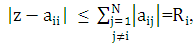 | (3.1) |
where z is a complex number,  are the diagonal entries,
  are the non-diagonal entries and
  is a closed disc centered at
  with radius R. If all disks of the matrix A are contained in the unit circle of the complex plane, so do the eigenvalues and we will have stability [4].
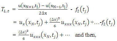
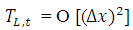
3.1. Consistency of the Explicit (FTCS) Scheme
Using equation (2.3) above and assuming that the true solution is smooth,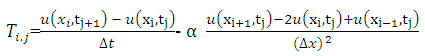 | (3.2) |
With a Taylor expansion,  Since
Since  then;
then; 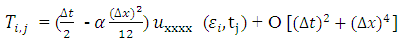 Where,
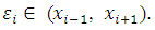
 | (3.3) |
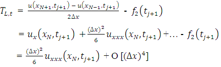
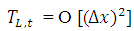
Therefore, the difference approximation is consistent at interior points. Again, the local truncation error (LTE) of the numerical boundary conditions at two boundary points 0 and L can be obtained as;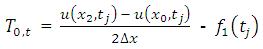 | (3.4) |
With a Taylor series expansion, 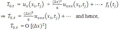 | (3.5) |
 | (3.6) |
 | (3.7) |
Since  and
and  will be used to calculate
  and
and  respectively, the TE at the boundary will spread in to the interior nodes. To see how this will affect the LTE there, we use equation (2.8) and (2.9) above to obtain the effective difference scheme on the nodes
  and
and  respectively.
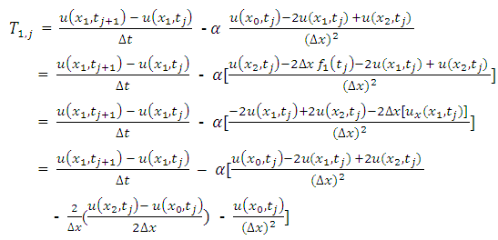 | (3.8) |
Then from Taylor series expansion, 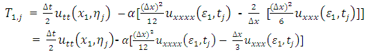 | (3.9) |
Where, 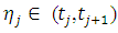 and
and  . Hence,
  as
as  .
. | (3.10) |
 | (3.11) |
Hence,  , as
, as  . Therefore, the difference approximation is consistent at the boundary points and the interior points.
3.2. Stability of the Explicit (FTCS) Scheme
For stability of FTCS scheme, it is suffices to show that the eigenvalues of the coefficient matrix A of equation (2.12) are contained in circles centered at (1-2r) with radius of 2r. 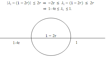 But, for stability
 , so that for
  is satisfied.For
 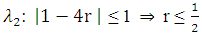 . Therefore, the explicit scheme is stable if
  .
.
3.3. Consistency of the Implicit (BTCS) Scheme
Using equation (2.15),  | (3.12) |
Using a Taylor series expansion, Recall that,
  such that;
 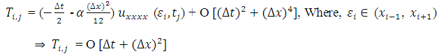 | (3.13) |
And, the LTE of the numerical boundary conditions becomes, 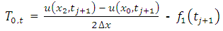 | (3.14) |
By Taylor series expansion, 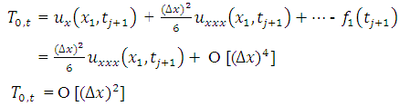 | (3.15) |
 | (3.16) |
 | (3.17) |
The effective difference scheme on the nodes  and
and  become,
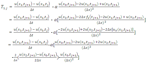 | (3.18) |
Then from Taylor series expansion, 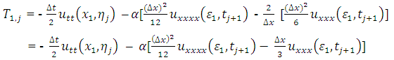 | (3.19) |
Where,  and
and 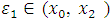 . Hence,
  , as
, as  . Again,
 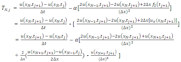 | (3.20) |
 | (3.21) |
Hence,  , as
, as  .Therefore, the difference approximation is consistent at the boundary points and the interior points.
3.4. Stability of the Implicit (BTCS) Scheme
Using Gerschgorin’s Theorem, the eigenvalues of the coefficient matrix A of equation (2.22) are contained in circles centered at (1+2r) with radius of 2r. 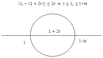 Thus, all eigenvalues are at least 1. In solving for
  in equation (2.23), we have
 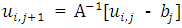 . Since the eigenvalues of A-1 are the reciprocal of the eigenvalues of A, the eigenvalues of A-1 are all ≤ 1. Thus, the implicit algorithm yields stable iterates and do not grow without bound. Hence, it is unconditionally stable.
4. Numerical Experiments and Discussion
This section presents convergence rates of the FTCS and BTCS schemes by means of applying the schemes to solve a one dimensional diffusion equation with Neumann boundary conditions. Four numerical problems are presented and, both FTCS and BTCS schemes have been implemented on the same time steps for each iteration solution. To look at the accuracy of the methods, difference between the exact solution  and the approximate solution
  (solution error) is used. For
  denotes the error in the calculation with grid spacing
  , its magnitude is measured by the maximum norm,
  | (4.1) |
To improve the accuracy and again to determine order of accuracy of the methods, the grid sizes were refined. The time step size  is set extremely small to reduce the effect from the temporal dimension, so that the discretization error in time is negligible in which we have used,
  | (4.2) |
k = 1, 2, 3, 4, 5, 6 (which is the number of iterations), to have a proper resolution expecting that the resulting error of the solution will approaches to zero. Then, we plot numerical solutions with their exact solutions for different iterations to determine convergence of the methods as grid sizes were refined. The order of accuracy p which determines convergence rate between two errors, [3, 8] was obtained as,  | (4.3) |
We also plot errors as a function of  in a loglog plot and determine the slope of the line that appears to approximate p. In this work, we have taken thermal diffusivity constant
  , total number of spatial nodes for first iteration N = 6 for the interval [0, 1] which means
  , total number of time steps for first iteration M = 51 for the interval [0, 1] which means
  . Example 1: Consider one dimensional heat equation
  with initial condition
  , and boundary conditions
 The exact solution is given by
  .The numerical results of the example are shown in Figure 1, Table 1 and Figure 2 below.
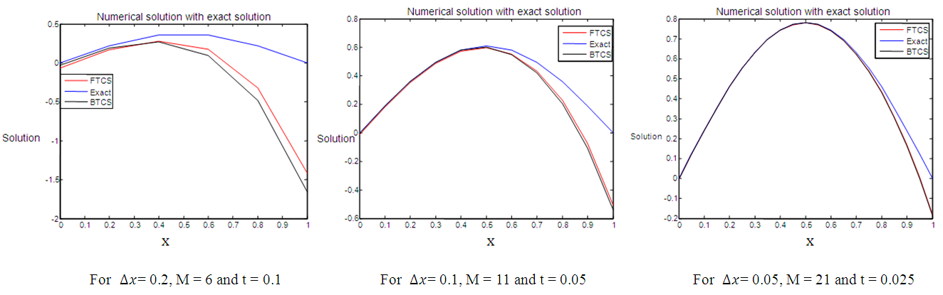 | Figure 1. FTCS and BTCS solutions with their exact solutions for example 1 |
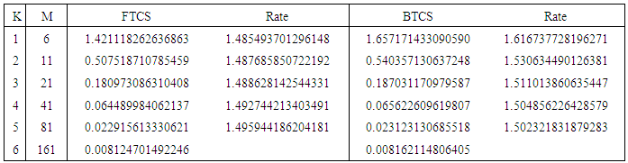
Table 1. Convergence rate of FTCS and BTCS schemes for example 1
 |
| |
|
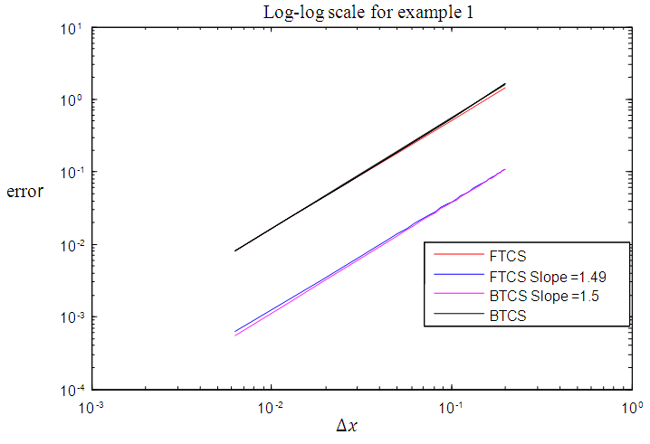 | Figure 2. Order of accuracy of FTCS and BTCS methods for example 1 |
Example 2: Consider one dimensional heat equation  with initial condition
  , and boundary conditions
 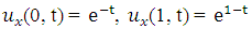 .The exact solution is given by
 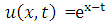 . The numerical results of the example are shown in Figure 3, Table 2 and Figure 4 below.
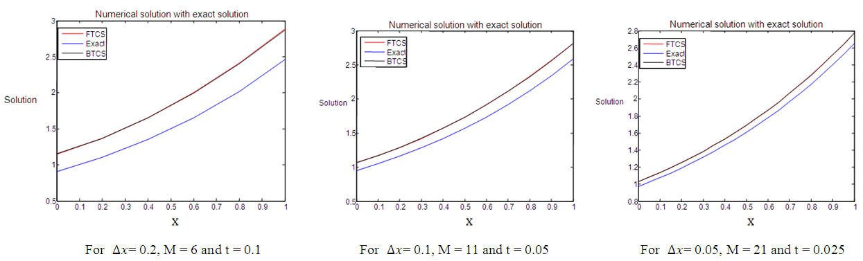 | Figure 3. FTCS and BTCS solutions with their exact solutions for example 2 |
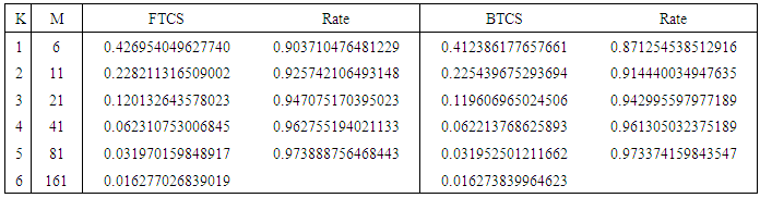
Table 2. Convergence rate of FTCS and BTCS schemes for example 2
 |
| |
|
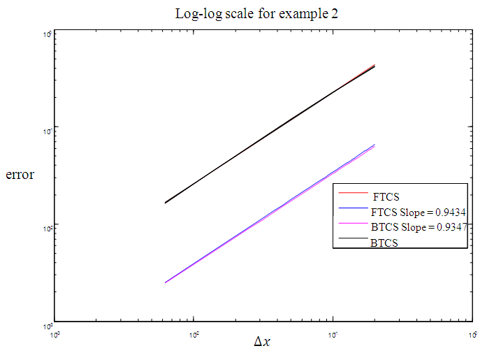 | Figure 4. Order of accuracy of FTCS and BTCS methods for example 2 |
Example 3: Consider one dimensional heat equation  with initial condition
 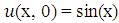 , and boundary conditions
  .The exact solution is given by
  .The numerical results of the example are shown in Figure 5, Table 3 and Figure 6 below.
 | Figure 5. FTCS and BTCS solutions with their exact solutions for example 3 |
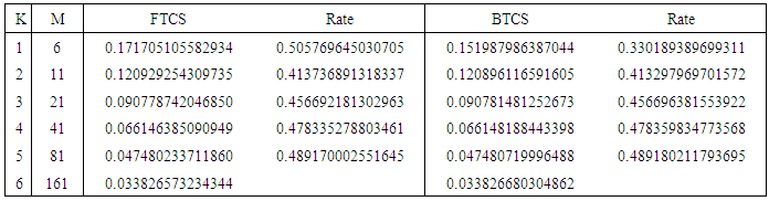
Table 3. Convergence rate of FTCS and BTCS schemes for example 3
 |
| |
|
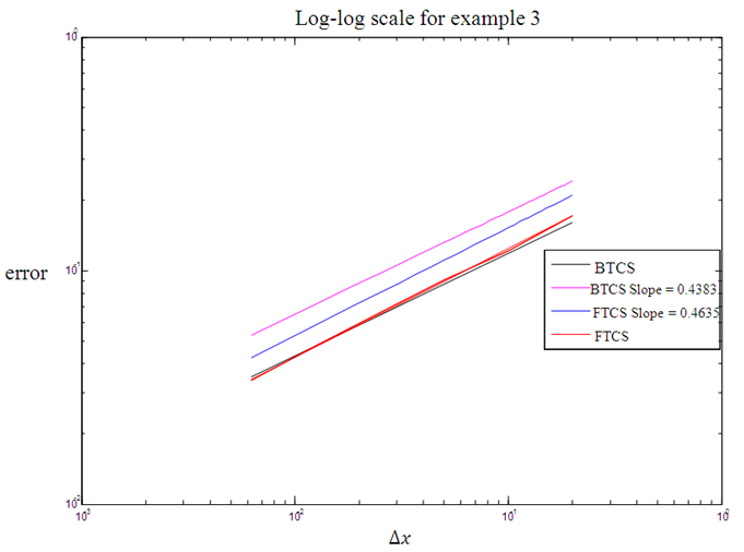 | Figure 6. Order of accuracy of FTCS and BTCS methods for example 3 |
Example 4: Consider inhomogeneous one dimensional heat equation 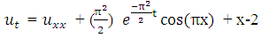 with initial condition
 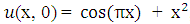 , and boundary conditions
 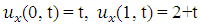 .The exact solution is given by
 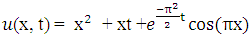 .The numerical results of the example are shown in Figure 7, Table 4 and Figure 8 below.
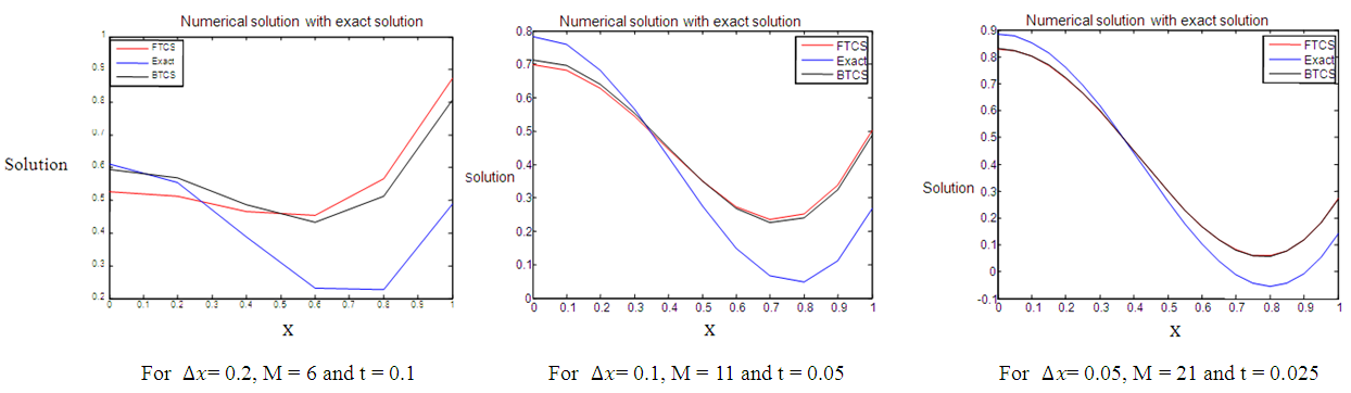 | Figure 7. FTCS and BTCS solutions with their exact solutions for example 4 |
Table 4. Convergence rate of FTCS and BTCS schemes for example 4
 |
| |
|
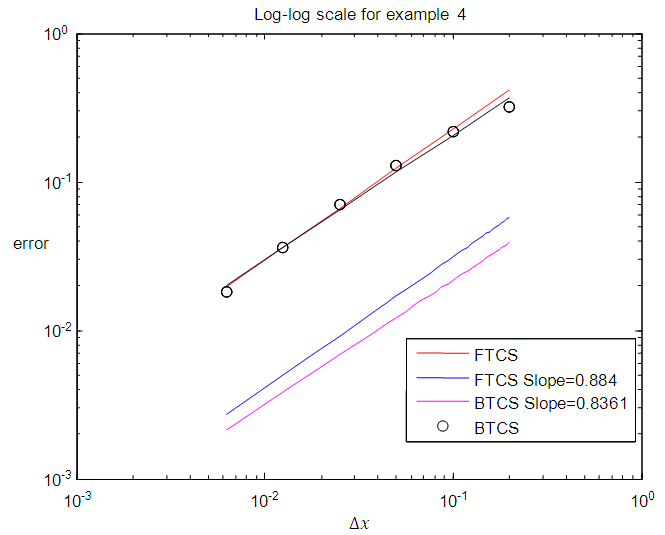 | Figure 8. Order of accuracy of FTCS and BTCS methods for example 4 |
Figure 1, Figure 3, Figure 5 and Figure 7 above present the numerical solutions with their exact solutions for each example and clearly show that the methods are convergent as grid sizes were refined. Also as one can see from the error values computed in the Table 1 – Table 4, as grid sizes were refined the error of the two methods reduces and becomes almost the same with one another which indicates that, solutions of the methods are very similar and also accurate, smooth and hardly distinguishable from the exact solution. Also both methods are first-order accurate in the spatial dimension. But their convergence rate towards its order of accuracy is slow in every Table. This first order of accuracy can be obtained by the effect of using Neumann boundary conditions at end points  and
and  in which the errors in the ratio of differences to find order of accuracy prevents the convergence rate to be actual order.
5. Conclusions
This study has considered the FTCS and BTCS finite difference schemes for solving one dimensional time dependent diffusion equation with Neumann boundary conditions. The difference schemes are derived. Using Lax Equivalence Theorem, convergence of the methods was described by testing consistency and stability of the methods. Stability was discussed by using Gerschgorin’s Theorem and shown that BTCS method is unconditionally stable and FTCS method is stable only if stability limit  . A systematic study was applied to the four test numerical problems and the schemes have been successfully applied. The performance of the schemes for the considered problems was measured by calculating the error. The result of the computed errors showed that, increasing of resolution increases accuracy of the methods and therefore schemes are capable of solving the problems. Most usefully the analysis presented here shows that, both methods are first-order accurate in the spatial dimension regardless of the actual order by the result of using Neumann boundary conditions.
References
| [1] | Khosro Sayevand, Convergence and stability analysis of modified backward time centered space approach for non-dimensionalizing parabolic equation, J. Nonlinear Sci. Appl. 7 (2014), 11-17. |
| [2] | Ramandeep Kaur, Numerical Solutions and Stability of Some Partial Differential Equations Using Finite Difference Methods, Roll No: 301103015, MSc Thesis, Thapar University, Patiala-147004 (Punjab) INDIA, June 2013. |
| [3] | Randall J. LeVeque, Finite Difference Methods for Diffusion Equations. DRAFT VERSION for use in the course A Math 585 – 586, University of Washington, version of September, 1998. |
| [4] | Michael H. Mkwizu, The stability of the one space dimension Diffusion Equation with Finite Difference Methods, M.Sc. (Mathematical Modelling) Dissertation, University of Dar es Salaam, August 2011. |
| [5] | Mark Davis, Finite Difference Methods, Department of Mathematics, MSc Course in Mathematics and Finance, Imperial College London, 2010-11. |
| [6] | M. Akram, On Numerical Solution of the Parabolic Equation with Neumann Boundary Conditions, International Mathematical Forum, 2, 2007, no. 12, 551 – 559. |
| [7] | S. Mishra and N. Risebro, and F. Weber, Convergence rates of finite difference schemes for the wave equation with rough coefficients, Research Report No. 2013-42, Seminar for Applied Mathematics, ETH Z¨urich, Switzerland, 2013. |
| [8] | S.L. Mitchell, M. Vynnycky, Finite-difference methods with increased accuracy and correct initialization for one-dimensional Stefan problems, Applied Mathematics and Computation 215 (2009) 1609–1621. |

 Abstract
 Reference
 Full-Text PDF
 Full-text HTML