J. Sunday 1, A. A. James 2, M. R. Odekunle 3, A. O. Adesanya 3
1Department of Mathematics, Adamawa State University, Mubi, Nigeria
2Mathematics Division, American University of Nigeria, Yola, Nigeria
3Department of Mathematics, Modibbo Adama University of Technology, Yola, Nigeria
Correspondence to: J. Sunday , Department of Mathematics, Adamawa State University, Mubi, Nigeria.
| Email: |  |
Copyright © 2016 Scientific & Academic Publishing. All Rights Reserved.
This work is licensed under the Creative Commons Attribution International License (CC BY).
http://creativecommons.org/licenses/by/4.0/

Abstract
Damping is an influence within or upon an oscillatory system that has the effect of reducing, restricting or preventing its oscillations. A one-step sixth-order computational method is proposed in this paper for the solution of second order free undamped and free damped motions in mass-spring systems. The method of interpolation and collocation of power series approximate solution was adopted to generate a continuous computational hybrid linear multistep method which was evaluated at grid points to give a continuous block method. The resultant discrete block method was recovered when the continuous block method was evaluated at selected grid points. The basic properties of the method was also investigated and found to be zero-stable, consistent and convergent.
Keywords:
Computational Approach, Damping, Free Damped Motion, Free Undamped Motion, Mass-Spring Systems
Cite this paper: J. Sunday , A. A. James , M. R. Odekunle , A. O. Adesanya , Solutions to Free Undamped and Free Damped Motion Problems in Mass-Spring Systems, American Journal of Computational and Applied Mathematics , Vol. 6 No. 2, 2016, pp. 82-91. doi: 10.5923/j.ajcam.20160602.08.
1. Introduction
In physical systems, damping is produced by processes that dissipate the energy stored in the oscillation. Examples include viscous drag in mechanical systems, resistance in electronic oscillators, and absorption and scattering of light in optical oscillators. Damping not based on energy loss can be important in other oscillating systems such as those that occur in biological systems. The damping of a system can be described as being one of the following;- Overdamped: the system returns (exponentially decays) to equilibrium without oscillating- Critically damped: the system returns to equilibrium as quickly as possible without oscillating- Underdamped: the system oscillates (at reduced frequency compared to the undamped case) with the amplitude gradually decreasing to zero- Undamped: the system oscillates at its natural resonant frequency As a practical example, consider a door that uses a spring to close the door once open. This can lead to any of the above types of damping. If the door is undamped, it will swing back and forth forever at a particular resonant frequency. If it is underdamped, it will swing back and forth with decreasing size of the swing until it comes to a stop. If it is critically damped, then it will return to closed as quickly as possible without oscillating. Finally, if it is overdamped, it will return to closed without oscillating but more slowly depending on how overdamped it is. We shall state two very important laws as regards to mass-spring systems.Hooke’s Law: states that the restoring force  exerted by a spring when it is stretched or compressed is proportional to the distance
  that it is stretched or compressed. That is,
  , where the constant of proportionality
  is called the spring constant.Newton’s Second Law: states that suppose
  be the mass of a body,
  the resultant force acting upon it and
  be the acceleration produced in the body. Then, by Newton’s second law, we have
  .In this paper, a one-step sixth-order computational method for the solution of second order free undamped and free damped motions in mass-spring systems of the form,
 | (1) |
shall be considered, where  is continuous within the interval of integration.Direct methods for the solution of higher-order ODEs have been proposed by many authors and they concluded that direct methods are more convenient and accurate than the method of reduction to systems of first order ODEs, [8]. Some of the authors that proposed direct methods include [1], [6], to mention a few. These authors proposed continuous implicit linear multistep methods which were implemented in predictor-corrector mode where they developed reducing order predictors to implement the corrector. The authors in [2] reported that one of the setbacks of predictor-corrector method is that it is very costly to implement as subroutine are very complicated to write because it requires special technique to supply the starting values and varying step size leads to longer computer time and human efforts. Above all, the predictors are in reducing order; hence it affects the accuracy of the method. The author [5] reported that continuous linear multistep method has greater advantages over the discrete method in that it gives better error estimation, provide a simplified coefficient for further analytical work at different points and guarantee easy approximation of solution at all interior points within the interval of integration. Scholars later developed block methods to cater for some of the setbacks of predictor-corrector methods mentioned above. Block method generates independent solution at selected grid point without overlapping. It is less expensive in terms of the number of function evaluation compared to predictor- corrector method; moreover it possesses the properties of Runge-Kutta method for being self-starting and does not require starting values. Some of the authors that proposed block methods are [3], [4], [12], among others.
2. The Differential Equation of the Vibrations of Mass-Spring Systems
Let  be the natural (unstretched) length of a coil spring. Suppose a mass
  is attached to the lower end of the spring so that it comes to rest in its equilibrium position
  , this stretches the spring by an amount
  , so that the stretched length is
  . At the equilibrium position
  , the mass
  is acted upon by two forces i.e. the weight
  acting vertically downwards and the spring force
  acting vertically upwards. Thus, we have
 | (2) |
Supposing  is the position of the mass (below equilibrium position) at any time
  so that the distance from the equilibrium position
  to the point
  is given by
  . Then
  may be positive, zero or negative according to whether the mass is below, at, or above its equilibrium position.When the mass is situated at
  , it is acted upon by the following forces. The forces tending to pull the mass downward are positive, while those pulling it vertically upward are negative.(i)
  , acting in the vertically downward direction(ii) Let
  be the restoring force of the spring. When the mass is at
  ,
,  is acting in the upward direction and so it is negative. By Hooke’s law, we have
 | (3) |
Using (2) in (3), we get | (4) |
(iii) Let  be the resisting force of the medium called damping force. It is known that for small velocities,
  is approximately proportional to the magnitude of the velocity. When the mass moving downward (at
  , say),
  acts in the upward direction (opposite to that of the motion) and so
  is negative and is given by,
 | (5) |
(iv) External impressed force  acting in downward direction.By Newton’s second law,
 | (6) |
where  and
and  . Thus,
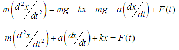 | (7) |
which is a differential equation for the motion of the mass on a spring and is of the form (1). If  , the motion is called undamped otherwise it is called damped. If there are no external impressed forces,
  for all
  , the motion is called free, otherwise it is called forced, see [13].
3. Methodology
In deriving the new one-step sixth-order computational method for the solution of free undamped and free damped problems of the form (1), power series basis function of the form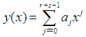 | (8) |
shall be considered. Here,  are the numbers of interpolation and collocation points respectively. Differentiating (8) twice, we get
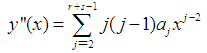 | (9) |
Substituting (9) into (1) gives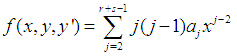 | (10) |
Interpolating (8) at 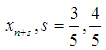 and collocating (10) at
 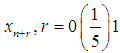 gives a system of non linear equation of the form,
 | (11) |
where 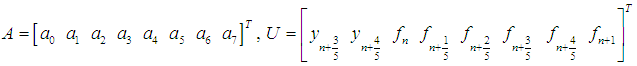 and
and 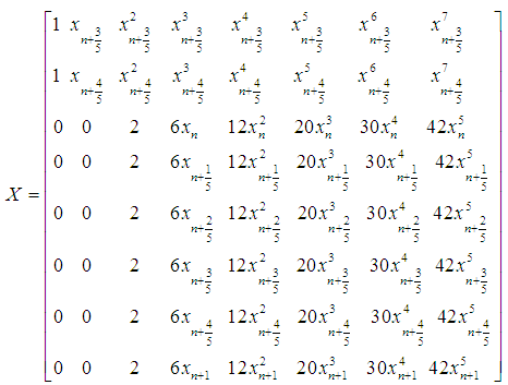 Solving (11), for
  using Gaussian elimination method and substituting into (8) gives a continuous hybrid linear multistep method of the form,
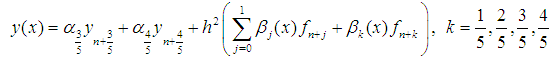 | (12) |
The coefficients of 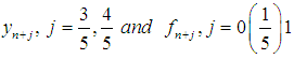 give,
give,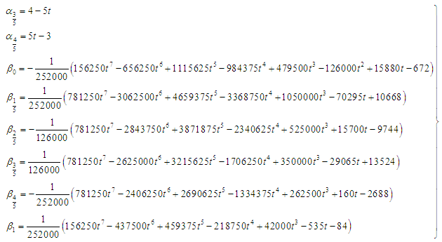 | (13) |
where 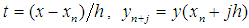 and
and  . Solving (12) for the independent solution at the grid points gives the continuous block method,
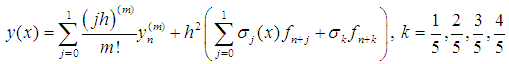 | (14) |
The coefficients of 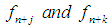 give,
give,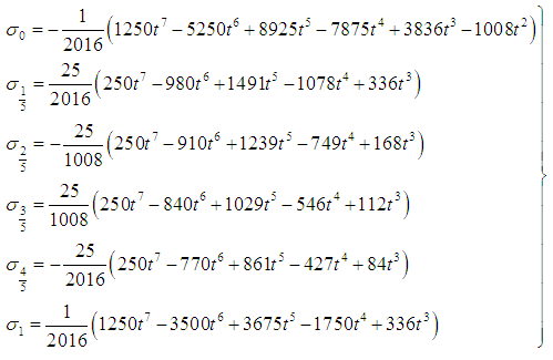 | (15) |
Evaluating (14) at  gives a discrete one-step computational block method of the form,
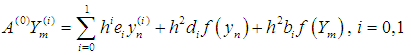 | (16) |
where 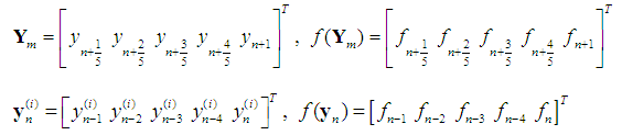 and
and  identity matrix.When
  :
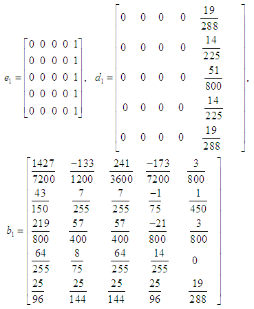
: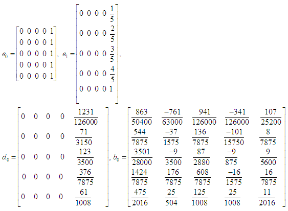 When
When  :
:
4. Analysis of Basic Properties of the Computational Method
4.1. Order of the Computational Method
Let the linear operator  associated with the discrete computational block method (16) be defined as,
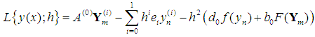 | (17) |
Expanding (17) in Taylor series and comparing the coefficients of  gives,
 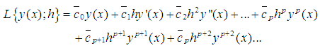 | (18) |
Definition 1 [11]: The linear operator  and the associated block formula (16) are said to be of order
  if
if 
 is called the error constant and implies that the local truncation error is given by,
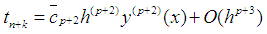 | (19) |
Expanding the newly derived computational method in Taylor series gives,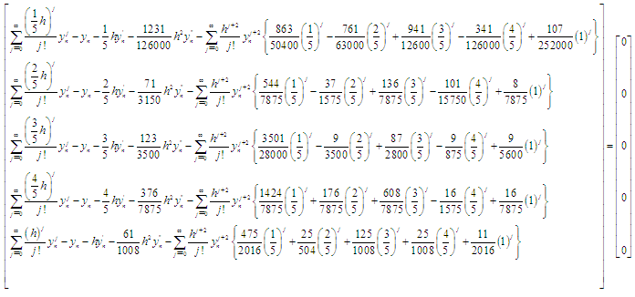 | (20) |
Comparing the coefficients of  gives
gives  and the error constant is given by
  Therefore, the computational method is of uniform order six.
4.2. Zero Stability of the Computational Method
Definition 2 [10]: The block method (16) is said to be zero-stable, if the roots  of the first characteristic polynomial
  defined by
 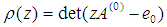 satisfies
  and every root satisfying
  have multiplicity not exceeding the order of the differential equation. Moreover, as
 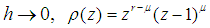 where
where  is the order of the differential equation,
  is the order of the matrices
  , see [7] for details. For our computational method,
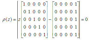 | (21) |
 . Hence, the computational method is zero-stable.
4.3. Consistency of the Computational Method
The computational block method (16) is consistent since it has order  .
.
4.4. Convergence of the Computational Method
The computational method is convergent by consequence of Dahlquist theorem stated below.Theorem 1 [9]: The necessary and sufficient conditions that a continuous LMM be convergent are that it be consistent and zero-stable.
4.5. Region of Absolute Stability of the Computational Method
Definition 3 [14]: Region of absolute stability is a region in the complex  plane, where
  . It is defined as those values of
  such that the numerical solutions of
  satisfy
  for any initial condition.We shall adopt the boundary locus method to determine the region of absolute stability of the computational method. This gives the stability polynomial,
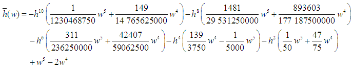 | (22) |
This gives the stability region shown in the figure below.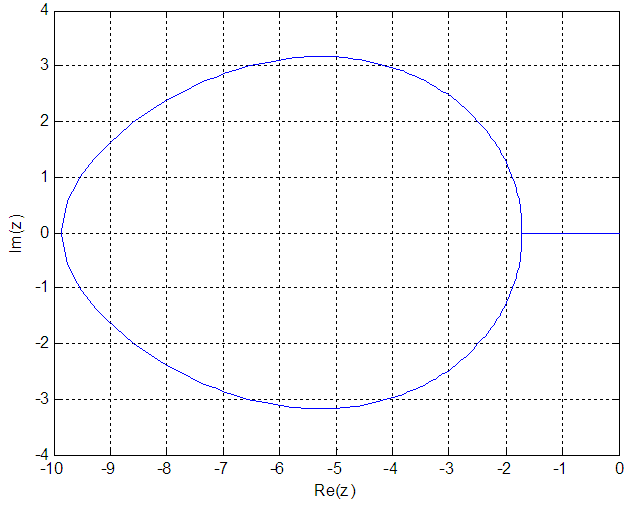 | Figure 1. Region of Absolute Stability of the One-Step Sixth-Order Computational Method |
By virtue of the figure obtained above, the stability region is A-stable, see [11] for details.
5. Numerical Experiments and Results
We shall test the performance of the one-step sixth-order computational method developed on two problems, i.e. the free undamped and free damped motions in mass-spring systems. Problem 1 (Free Undamped Motion)An  weight is placed upon the lower end of a coil spring suspended from the ceiling. The weight comes to rest in its equilibrium position, thereby stretching the spring
  . The weight is then pulled down
  below its equilibrium position and released at
  with an initial velocity of
  directed downwards. Neglecting the resistance of the medium and assuming that no external forces are present, determine the resulting motion of the weight on the spring at time
  .Source: [13]Analysis: the natural length of the spring
  . The mass
  slugs is attached to its lower end, thereby stretching the spring by an amount
  . In the position of equilibrium, the mass is acted upon by two forces:(i)
  (the weight) acting in the vertically downward direction(ii) the restoring force (spring force)
  acting in the vertically upwards, see equation (4). Thus,
  On applying equation (6), we get
 which results to,
 | (23) |
Since the weight was released with a downward initial velocity  from a point
  below its equilibrium position O, we have the following initial conditions as:
  So that the second order differential equation modeling the free undamped problem becomes,
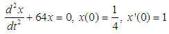 | (24) |
with the exact solution,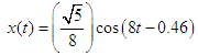 | (25) |
Problem 2 (Free Damped Motion)An  weight is attached to the lower end of a coil spring suspended from the ceiling. The weight comes to rest in its equilibrium position, thereby stretching the spring
  . The weight comes to rest in its equilibrium position, thereby stretching the spring
  . The weight is then pulled down
  below its equilibrium position and released at
  . No external forces are present, but the resistance of the medium is numerically equal to
  , where
  is the instantaneous velocity in feet per second. Determine the resulting motion of the weight on the spring at time
  .Source: [13] Analysis: here,
  the elongation of the spring after the weight is attached
  . Using Hooke’s law, we have
 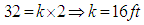 . Again,
  so that
  . Here, damping factor
  Using these facts, the basic differential equation of the vibration of the given mass on spring for the free damped motion given by equation (7) reduces to,
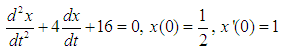 | (26) |
with the exact solution,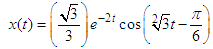 | (27) |
5.1. Discussion of Results
It is important to note that,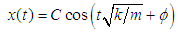 | (28) |
describes the free vibrations or free motion of a mechanical system (free of external influencing forces other than those imposed by gravity and the spring itself). Note that  is called the amplitude of the motion and gives the maximum (positive) displacement of the mass from the point
  . The motion is a periodic motion and the mass oscillates back and forth between
  .
.  is the spring constant and
  the mass.The time interval
  between two successive maxima is called the period of the motion and is given by
  . The reciprocal of the period, which gives the number of oscillation per second is called the natural frequency (or simply frequency) of the motion. The number
  is called the phase constant (or phase angle).For problem 1 (free undamped motion), the amplitude of the motion is
  , the period
  and the frequency is
  i.e.
i.e.  oscillations/sec. Free undamped motions are usually called simple harmonic motion.For problem 2 (free damped motion), the damping factor is
  , the period is
  .
.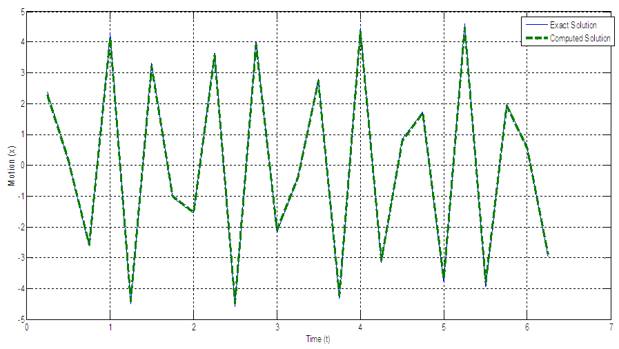 | Figure 2. Graphical Result for free undamped motion (problem 1) |
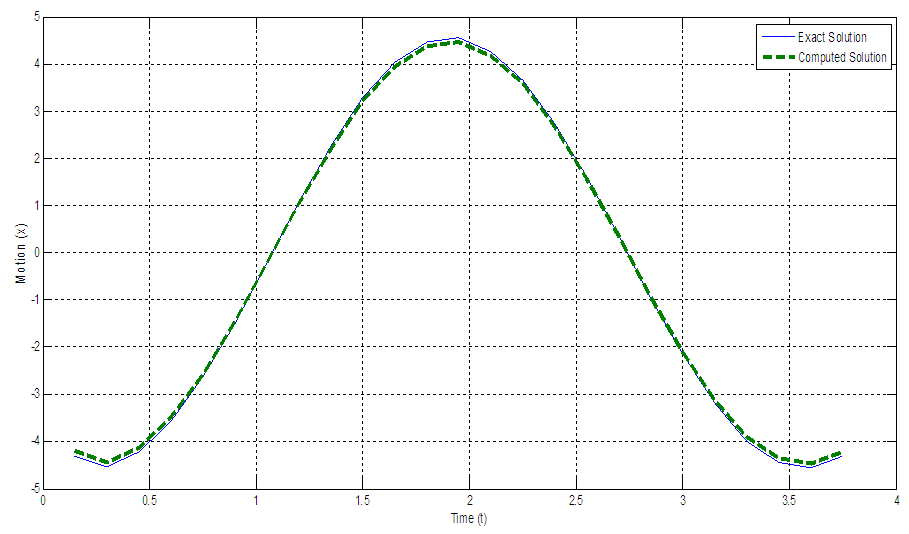 | Figure 3. Graphical Result for free damped motion (problem 2) |
Generally, from the graphical plots presented in Figures 2 and 3, one can say that the computed solutions converge toward the exact solutions for the two problems considered. Thus, the method can be said to be consistent, convergent, stable and computationally reliable.
6. Conclusions
We developed a one-step sixth-order computational method for free damped and free undamped systems for second order differential equations. From the graphical results obtained and the analysis carried out, it is obvious that the method is computationally reliable. The method has also been shown to be convergent, consistent and stable. Furthermore, the stability region of the method shows that it is A-stable; implying that it can efficiently cope with oscillatory and stiff problems. Finally, it is important to state that this method does not only compute motions in mass-spring systems but can efficiently solve any real-life problem that can be modeled into second order differential equation of the form (1).
References
| [1] | A. O. Adesanya, T. A. Anake, and M. O. Udoh, Improved Continuous Method for Direct Solution of General Second Order ODEs, Journal of Nigerian Association of Mathematical Physics, 3, 59-62, 2008. |
| [2] | A. O. Adesanya, M. R. Odekunle, and M. A. Alkali, Three-steps Block Predictor-Block Corrector Method for Solution of General Second Order ODEs, International Journal of Engineering Research and Applications, 2(4), 2297-2301, 2012. |
| [3] | A. O. Adesanya, M. A. Alkali and J. Sunday, Order Five Hybrid Block Method for the Solution of Second Order ODEs, International J. of Math. Sci. & Engineering Applications, 8(3), 285-295, 2014. |
| [4] | T. A. Anake, D. O. Awoyemi, and A. O. Adesanya, A One-step Method for the Solution of General Second Order ODEs, International Journal of Science and Engineering, 2(4), 159-163, 2012. |
| [5] | D. O. Awoyemi, A Class of Continuous Method for General Second Order IVPs in ODEs, International Journal of Computational Mathematics, 72, 29-37, 1999. |
| [6] | D. O. Awoyemi, A new sixth algorithm for General Second Order Ordinary Differential Equations, International Journal of Computational Mathematics, 77, 117-124, 2001. |
| [7] | D. O. Awoyemi, R. A. Ademiluyi, and W. Amuseghan, Off-grids Exploitation in the Development of More Accurate Method for the Solution of ODEs, Journal of Mathematical Physics, 12, 379-386, 2007. |
| [8] | D. O. Awoyemi, A P-stable Linear Multistep Method for Solving General Third Order ODEs, International Journal of Computational Mathematics, 80(8), 987-993, 2008. |
| [9] | G. G. Dahlquist, Convergence and Stability in the Numerical Integration of Ordinary Differential Equations, Math. Scand., 4, 33-50, 1956. |
| [10] | S. O. Fatunla, Numerical Methods for Initial Value Problems in Ordinary Differential Equations, Academic Press Inc, New York, 1988. |
| [11] | J. D. Lambert, Computational Methods in Ordinary Differential Equations, John Willey and Sons, New York, 1973. |
| [12] | K. M. Owolabi, A Family of Implicit Higher Order Methods for the Numerical Integration of Second Order ODEs, Mathematical Theory & Modeling, 2(4), 67-75, 2012. |
| [13] | M. D. Raisinghania, Ordinary and Partial Differential Equations, S. Chand and Company LTD, New-Delhi-110055, Revised Edition, 2014. |
| [14] | Y. L. Yan, Numerical Methods for Differential Equations, City University of Hong Kong, Kowloon, 2011. |

 Abstract
 Reference
 Full-Text PDF
 Full-text HTML