Harouna Naroua
Département de Mathématiques et Informatique, Université Abdou Moumouni, Niamey, Niger
Correspondence to: Harouna Naroua, Département de Mathématiques et Informatique, Université Abdou Moumouni, Niamey, Niger.
| Email: |  |
Copyright © 2016 Scientific & Academic Publishing. All Rights Reserved.
This work is licensed under the Creative Commons Attribution International License (CC BY).
http://creativecommons.org/licenses/by/4.0/

Abstract
In this paper, we make use of numerical methods in order to compute the solution of a fluid flow problem. For the purpose of application, we consider the unsteady flow of a viscous incompressible fluid occupying a semi-infinite region of space bounded by an infinite horizontal moving hot plate in the presence of indirect natural convection by way of an induced pressure gradient. Thermal radiation is taken into account in the problem. Computer programs based on a generic finite difference scheme and the Galerkin finite element method are employed to solve the coupled non-linear differential equations for velocity and temperature fields and the results of the two methods compared very well. The effects of thermal radiation as well as the other parameters entering into the problem are discussed extensively and shown graphically.
Keywords:
Computer Simulation, Generic Software Tool, Finite Element Method, Finite Difference Scheme, Unsteady Flow
Cite this paper: Harouna Naroua, A Comparative Analysis of a Thermal Radiative Flow of an Optically Thick Gray Gas in the Presence of Indirect Natural Convection, American Journal of Computational and Applied Mathematics , Vol. 6 No. 2, 2016, pp. 31-37. doi: 10.5923/j.ajcam.20160602.02.
1. Introduction
The study of fluid flows has important applications in engineering. For example, high temperature thermal radiation of an optically thin gray gas experiences a real life problem where nuclear effect does not involve reference to a homogeneous reaction of a non-catalytic system [1]. It finds wide applications in high temperature flight control and space technology. Various authors made important contributions in that field such as [1-8]. Both exact and numerical methods are used to solve fluid flow problems in various cases. Zhu et al. [9] analysed explicit/implicit schemes for parabolic equations with discontinuous coefficients. Numerical experiments, which were given for both linear and nonlinear problems, showed that their theoretical estimates are optimal in some sense. Naroua et al [10] presented a formulation coupling the classical finite element method with a stepwise Lagrange polynomial in order to compute the solution of a fluid flow problem. Instead of using line segments within elements as used by the classical method, they used polynomials of degree two over couples of elements. Matsuoka and Nakamura [11] proposed a stable numerical scheme for a Cahn-Hilliard type equation with long-range interaction describing the micro-phase separation of diblock copolymer melts. They designed their scheme by using the discrete variational derivative method which is one of the structure preserving numerical methods. They observed that their proposed scheme has the same characteristic properties, mass conservation and energy dissipation, as the original equation does. They also discussed the stability and unique solvability of their proposed scheme. Khader and Ahmed [12] introduced a numerical simulation using finite difference method with the theoretical study for the problem of the flow and heat transfer over an unsteady stretching sheet embedded in a porous medium in the presence of a thermal radiation.Although many improvements have been made in the use of numerical methods, we are proposing to compare a generic computer tool that we designed for that purpose with the finite element method on a specific non-linear problem. For the purpose of application, we consider the unsteady flow of a viscous incompressible fluid occupying a semi-infinite region of space bounded by an infinite horizontal moving hot plate in the presence of indirect natural convection by way of an induced pressure gradient. Thermal radiation is taken into account in the problem.
2. Mathematical Analysis
The problem considered is an unsteady flow of a viscous incompressible fluid occupying a semi-infinite region of space bounded by an infinite horizontal plate moving with constant velocity u0 with reference to indirect natural convection by way of an induced pressure gradient. The geometry and the unsteady flow fields for this problem are described by Ghosh and Pop [1] in which we used R in the place of the radiation parameter K1 for convenience. They assumed a flow of an optically thick gray gas with indirect natural convection and radiation. The x/ -axis is taken along the plate and the y/ -axis is normal to it as shown in Figure 1. 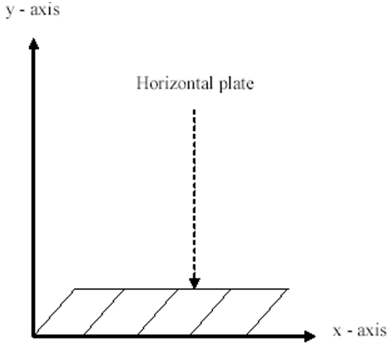 | Figure 1. The flow configuration |
The problem considered reduces to the following non-dimensional differential equations [1]: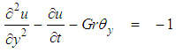 | (1) |
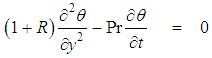 | (2) |
where- u is the dimensionless velocity,- Ө is the dimensionless temperature,- Gr is the Grashof number,- Pr is the Prandtl number,- R is the Radiation parameter.The boundary conditions are given as follows: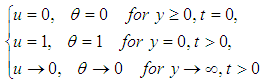 | (3) |
2.1. Solution of the Problem Using the Generic Software
The system of equations (1) and (2) with boundary conditions (3) has been solved numerically by a generic software using a finite-difference scheme as described by Nakamura [4]. The mesh system is shown in Figure 2. The numbers of spatial and temporal subdivisions are respectively I+1 and J+1. The steps in space and time are respectively represented by i and j.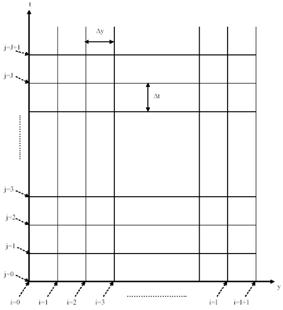 | Figure 2. Mesh system |
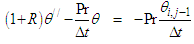
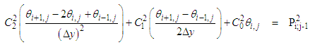
Equations (1) and (2) are coupled non-linear parabolic partial differential equations in u and Ө. We first discretize equations (1) and (2) using the backward difference approximation (which is stable) in the time coordinate as shown in equations (4) and (5):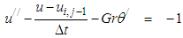 | (4) |
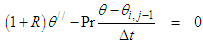 | (5) |
where  are derivatives with respect to y. The system of equations (4-5) can be rewritten as:
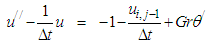 | (6) |
 | (7) |
For the sake of simplicity, we write: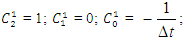
 Using the above formulation, equations (6-7) take the form:
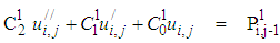 | (8) |
 | (9) |
Using the central difference scheme which is unconditionally stable, equations (8-9) reduce to: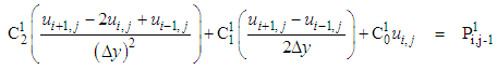 | (10) |
 | (11) |
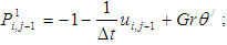
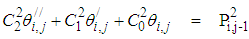
At time step j+1, equations (10-11) reduce to: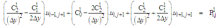 | (12) |
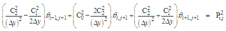 | (13) |
Equations (12-13) cannot be solved individually for each grid point i. The equations for all the grid points must be solved simultaneously. The set of equations for i = 1,2,...........,I forms a tridiagonal system of equations as described by Nakamura [4] and shown in equations (14-15).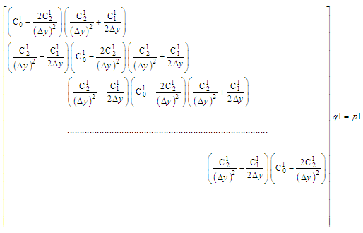 | (14) |
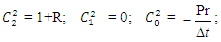
where 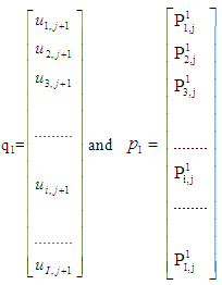
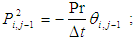
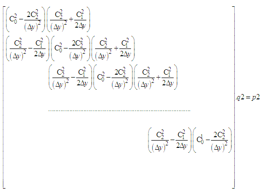 | (15) |
where 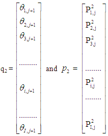 For each time step, the system of equations (14-15) requires an iterative procedure due to the presence of non-linear coefficients. Successive substitutions and iterations are continuously executed for each time step until convergence is reached.
2.2. Solution of the Problem Using the Finite Element Method
The initial system of equations (1-2) with boundary conditions (3) has been solved numerically by a computer program using the finite element method in step 1 and step 2.Step 1: Energy equation finite element formulationWe solve equation (2) with the help of boundary conditions (3). Constructing the quasi - variational equivalent of equation (2), we obtain: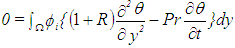 | (16) |
where  denotes the test function and
  is the region of the flow.Consider an N elements mesh and a two parameter (semi discrete) Galerkin approximation of the form [13]:
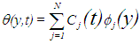 | (17) |
with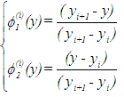 | (18) |
where i = 1,2,3,…,N and yi and yi+1 are respectively the lower and upper coordinates of the element i. Using equations (17-18), equation (16) reduces to: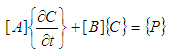 | (19) |
where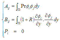 | (20) |
Using the Θ - family of approximation developed by Reddy [13], equation (19) reduces to: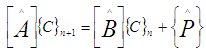 | (21) |
where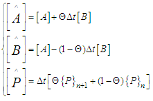 | (22) |
The initial value C0 is obtained by the Galerkin method from a 32 elements mesh and is given by: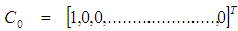 | (23) |
For t > 0,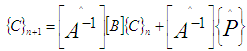 | (24) |
Step 2: Momentum equation finite element formulationWe solve equation (1) with the help of boundary conditions (3). Constructing the quasi - variational statement of equation (1), we obtain: 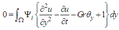 | (25) |
where Ψi is the test function and Ω is the region of the flow.Consider a two parameter (semi-discrete) Galerkin approximation of the form [13]: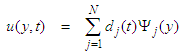 | (26) |
with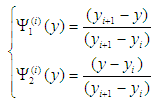 | (27) |
where i=1,2,3,…..,N and yi and yi+1 are respectively the lower and upper coordinates of the element i.Using equations (26-27), equation (25) reduces to: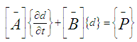 | (28) |
where | (29) |
Using the Θ - family of operators developed by Reddy [13], equation (28) takes the form: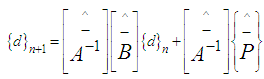 | (30) |
where | (31) |
The numerical values of the temperature and velocity fields have been computed from equations (24) and (30).
3. Discussion of Results
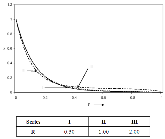
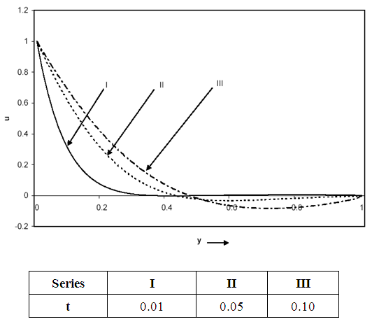
In order to achieve a physical understanding of the problem and for the purpose of discussing the results, numerical calculations have been carried out for the velocity and temperature distributions. The results obtained from the two methods showed insignificant differences and are graphically the same. Figures 3-9 are the same for both methods and are used for the analysis. The velocity profiles are examined for the cases Gr > 0 and Gr < 0. Gr > 0 (= +5) is used for the case when the flow is in the presence of cooling of the plate by free convection currents. Gr < 0 (= -5) is used for the case when the flow is in the presence of heating of the plate by free convection currents. Figures 3-8 show the velocity distribution for the two cases from which we observe that the velocity (u) decreases away from the plate.From Figures 3, 4 and 5, for the case when Gr>0 (in the presence of cooling of the plate by free convection currents), we observe that:i. The velocity (u) decreases due to an increase in the Prandtl number (Pr) while it increases due to an increase in the time (t).ii. An increase in the radiation parameter (R) leads to a fall in the velocity for y<0.32 while it leads to an increase in the velocity for y>0.32, which is in agreement with Ghosh and Pop [1].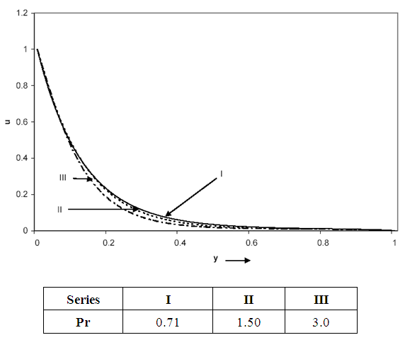 | Figure 3. Velocity distribution for Gr = 5, R = 0.5, t = 0.01 |
 | Figure 4. Velocity distribution for Gr = 5, Pr = 0.71, t = 0.01 |
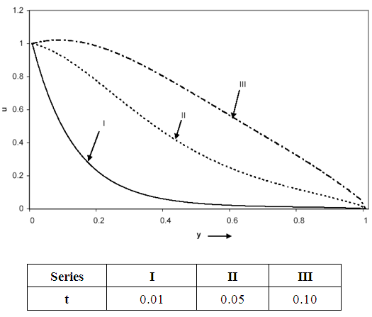 | Figure 5. Velocity distribution for Gr = 5, Pr = 0.71, R = 0.5 |
From Figures 6, 7 and 8, for the case when Gr<0 (in the presence of heating of the plate by free convection currents), we observe that:i. The velocity (u) increases due to an increase in the Prandtl number (Pr).ii. An increase in the radiation parameter (R) leads to an increase in the velocity (u) for y<0.32 while it leads to a fall in the velocity for y>0.32. The velocity is backward for y>0.32.iii. The velocity (u) increases with an increase in the time parameter (t) for yt while it decreases for y>yt where yt depends on t. The velocity can be backward far away from the plate.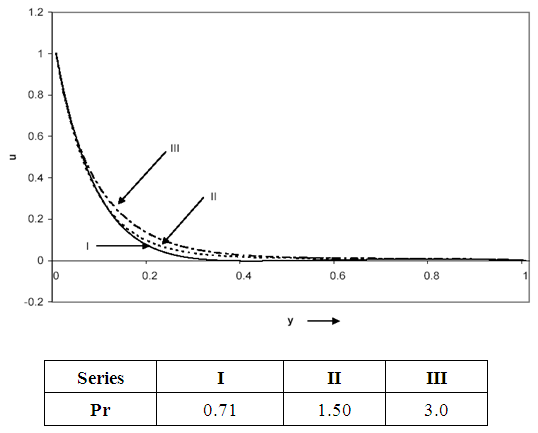 | Figure 6. Velocity distribution for Gr = -5, R = 0.5, t = 0.01 |
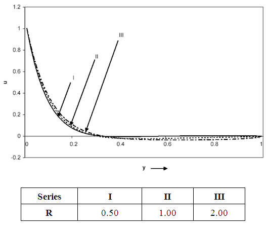 | Figure 7. Velocity distribution for Gr = -5, Pr = 0.71, t = 0.01 |
 | Figure 8. Velocity distribution for Gr = -5, Pr = 0.71, R = 0.5 |
From Figure 9, we observe that:i.The temperature (Ө) decreases away from the plate. The decrease is greater for a Newtonian fluid than it is for a non-Newtonian fluid (Ө decreases with Pr).ii.There is a rise in temperature profiles (Ө) due to an increase in the radiation parameter (R) and the time (t).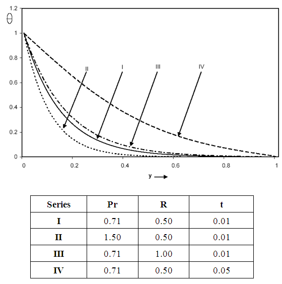 | Figure 9. Temperature distribution for Gr = ±5 |
References
| [1] | Ghosh, S. K. and Pop, I. (2007), Thermal radiation of an optically thick gray gas in the presence of indirect natural convection, International Journal of Fluid Mechanics Research, vol. 34, N°6, pp. 515-520. |
| [2] | Soundalgekar, V.M. and Takhar, H.S., (1980), “Combined forced and free convection MHD flow past a semi-infinite vertical plate’’, Wärmeund Stoffübertragung, vol. 14, pp. 153-158. |
| [3] | Bestman, A. R. and Adiepong, S. K. (1988), Unsteady hydromagnetic free-convection flow with radiative heat transfer in a rotating fluid, Astrophys. Space Sci., vol. 143, pp. 73-80. |
| [4] | Nakamura, S. (1991), Applied Numerical Methods with Software, Prentice-Hall International Editions. |
| [5] | Brewster, M. Q. (1992), Thermal radiative transfer and properties, John Wiley and Sons, New York. |
| [6] | Raptis A. and Massalas C.V. (1997), “Magnetohydrodynamic flow past a plate by the presence of radiation’’, Journal of Magnetohydrodynamics and Plasma Research, vol.7, n°2/3, pp. 121-128. |
| [7] | Yamauchi, J., Nakamura, S and Nakano H., (2000), “Application of Modified Finite-Difference Formulas to the Analysis of z-Variant Rib Waveguides’’, IEEE Photonics Technology Letters, vol 12, n°8, pp. 1001-1003. |
| [8] | Raptis, A. and Perdikis, C. (2003), Thermal radiation of an optically thin gray gas, Int. J. Appl. Mech. Engng, vol. 8, N°1, pp. 131-134. |
| [9] | Zhu, S., Yuan G. and Sun W., (2004), “Convergence and Stability of Explicit/Implicit Schemes for Parabolic Equations with Discontinuous Coefficients’’, International Journal of Numerical Analysis and Modeling, vol. 1, n°2, pp. 131–145. |
| [10] | Naroua, H., Takhar, H. S. and Slaouti, A. (2006), Computational challenges in fluid flow problems: a MHD Stokes problem of convective flow from a vertical infinite plate in a rotating fluid, European Journal of Scientific Research, vol. 13, N°1, pp. 101-112. |
| [11] | Matsuoka H. and Nakamura K-I., (2013), “A stable finite difference method for a Cahn-Hilliard type equation with long-range interaction’’, Sci. Rep. Kanazawa Univ., vol. 57, pp.13–34, 2013. |
| [12] | Khader, M.M. and Ahmed, M.M., (2013), “Numerical simulation using the finite difference method for the flow and heat transfer in a thin liquid film over an unsteady stretching sheet in a saturated porous medium in the presence of thermal radiation’’, Journal of King Saud University - Engineering Sciences, vol. 25, issue 1, pp. 29–34. |
| [13] | Reddy, J.N. (1984), An Introduction to the finite element method, Mc Graw Hill book company, Singapore. |

 Abstract
 Reference
 Full-Text PDF
 Full-text HTML