1. Introduction

Fractional differential equations (FDEs) are generalization of the classical differential equations of integer-order. Fractional derivatives are useful in describing the memory and hereditary-properties materials and processes. FDEs are widely used as models to express much important phenomena in natural science such as chemistry, biology, mathematics, communication, physics, engineering, diffusion process, porous media, power-law non-locality, and power-law long-term memory. The interested reader is also referred to numerous applications of fractional calculus in different areas of science [1-4]. The investigation of analytical and numerical solutions of FDEs became an important issue and matter of interest for researchers in the last decades. Many definitions of fractional integration and differentiation operators have been utilized. The Riemann-Liouville definition could be considered as a famous one [4], which has been applied successfully in various fields of science and engineering. However, it led to the result that the fractional derivative of a constant function is not zero. To overcome this problem, Caputo proposed a definition for differentiable functions that gave a zero value for constant function [4]. In addition, Caputo's definition is applicable to treat real-world phenomena modelled by FDEs. In the last few years, Jumarie modified the Riemann-Liouville derivative to new formulae that are suitable for continuous and non-differentiable functions, with a zero value derivative for a constant function [5-8]. The modified Riemann-Liouville fractional definition has been used effectively in various problems. There are many effective methods in the literature to treat FDEs such as the Adomian decomposition method, the variational iteration method, the homotopy perturbation method, the differential transform method, the finite difference method, the finite element method, the exponential function method, the fractional sub-equation method, the -expansion method, and the first integral method [9-27]. In this work, analytical solutions of the space-time fractional quantum Zakharov system for plasmas are studied based on fractional Riccati method, where the fractional derivatives are considered in sense of modified Riemann-Liouville derivative.

Quantum effects are expected to play a central role in the performance of today’s microelectronic devices, for which classical transport models are not always adequate in view of the increasing miniaturization level. Hence, the topic of quantum plasmas has recently attracted considerable attention, [28-38] and it is desirable to achieve a good understanding of the basic properties of quantum transport models. The importance of quantum effects can be estimated by considering the ratio of the thermal wavelength which characterizes the extension of the probability density of the plasma particles, to other characteristic lengths. Quantum effects are to be expected if: (1) the Landau length is of the same order as the thermal wavelength, i.e., and (3) the plasma particles are degenerated, i.e., with n being the density [28-38].

Soliton is a localized wave that arises from a balance between nonlinear and dispersive effects. In most types, the pulse width depends on the amplitude [39]. A soliton is a solitary wave that behaves like a "particle", in that it satisfies the following conditions: i) it must maintain its shape when it moves at constant speed; ii) when a soliton interacts with another soliton, it emerges from the "collision" unchanged except possibly for a phase shift. Bright soliton is a localized solitary wave that its tail can exactly vanish at infinity. Dark soliton is characterized as a localized intensity dip on a continuous wave (CW) background. Bright and dark solitons are the fundamental self-localized modes of the optical field in nonlinear dispersive media such as waveguides, optical fibers, and photonic crystals [39]. Bright solitons are characterized by a localized intensity peak on a homogeneous background, while dark solitons can be described by a localized intensity hole on a continuous wave background. Bright solitons are formed when the group-velocity dispersion in an optical fiber is anomalous (or, similarly, when the nonlinearity of a planar waveguide is self-focusing). In this case, the uniform carrier wave is unstable with respect to long-wave modulations allowing for the formation of solitons. This type of instability is known as the modulation instability [40]. On the contrary, dark solitons are formed in the case of normal group-velocity dispersion in fibers (or a self defocusing nonlinearity in waveguides), when a uniform carrier wave is modulationally stable. In the case of water waves, bright solitons are known to appear in the form of surface envelopes of modulated wave trains when the uniform carrier wave is modulationally unstable [40]. This happens for water depths above the modulation instability threshold, namely, at being the carrier wave number. In addition to theoretical predictions, envelope solitons were observed experimentally in Refs. [41]. Dark solitons can appear on shallow water below the modulation instability threshold, at [41]. Recently, they have been observed in a series of experiments performed in a water wave tank [42]. In mathematical terms, bright and dark solitons are described by the nonlinear Schrödinger equation (NLSE) of the focusing and defocusing types, respectively [42]. NLSE takes into account the second-order dispersion and the phase self-modulation (cubic nonlinear term). In the general context of weakly nonlinear dispersive waves, this equation was first discussed by Benney and Newell. In the case of gravity waves propagating on the surface of infinite-depth irrotational, inviscid, and incompressible fluid, NLSE was first derived by Zakharov [43]. The finite-depth NLSE was first derived by Hasimoto and Ono [44]. If the intensity of the dip is not zero, it is called gray soliton. Other types of solitons, W- and M-solitons, could be obtained [44]. The W-soliton can describe bright and dark solitary wave properties in the same expressions and its amplitude may approach a nonzero value when the x-variable approaches infinity. Li et al first presented the W-soliton to describe the propagation of femtosecond light pulses in an optical fiber. The M-soliton is composed of the product of bright and solitary waves, which was first proposed to describe the propagation of dark optical pulses in a finite-width background by Tian et al [44].

The structure of the paper is as follows: In section 2, some basic definitions and mathematical preliminaries of the fractional calculus theory are introduced. The fractional tanh function expansion method is investigated in section 3. The space–time fractional quantum Zakharov system is presented in section 4. Finally, some conclusions and discussions are given.

2. Mathematical Preliminaries

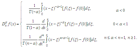
Fractional calculus is the generalizations of ordinary calculus. There are many kinds of fractional calculus. Such as Riemann–Liouville, Caputo, Kolwankar–Gangal, Oldham and Spanier, Miller and Ross, Cresson’s, Grunwald-Letnikov, and modified Riemann–Liouville [5-8, 45-53]. This work is motivated by the need to propose a fractional tanh function expansion method to construct exact analytical solutions of nonlinear FDEs with the modified Riemann–Liouville derivative defined by Jumarie [5-8] as follows

(1)

Owing to these merits, Jumarie’s modified-Riemann–Liouville derivative given by formula (1) was successfully applied to the probability calculus, fractional Laplace problems and fractional variational calculus. Some useful formulas and the results of Jumarie’s modified Riemann–Liouville derivative were summarized in [5-8], five of them are

(2)

(3)

(4)

(5)

(6)

where is constant. The formulae (4-6) are direct results from

(7)

Remark 1: He et. al. modified the chain rule Eq. (5) to the formula

(8)

where is called the fractal index which is usually determined in terms of gamma functions [45-46]. Therefore, equations (4) and (6) modified to the following forms

(9)

(10)

Throughout this manuscript, we use the relations (9-10) to solve the space–time fractional quantum Zakharov system, taking into consideration that the fractal index is unity [46].

Remark 2: Jumarie’s modified-Riemann–Liouville derivative for non-differentiable functions has similar rules and has mathematical limit definition comparable to certain definitions of local fractional derivatives introduced by Kolwankar–Gangal [47, 48], the Hausdorff derivative which is called fractal derivative [49-53] and the recently developed derivative [54-56].

3. Fractional Tanh Expansion Method

In this section, we outline the main steps of the fractional tanh function expansion method for solving nonlinear FDEs. For a given nonlinear FDE, say, in two variables

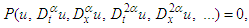(11)

where and are Jumarie’s modified-Riemann–Liouville derivatives of is an unknown function, is a polynomial in u and its various partial derivatives, in which the highest order derivatives and nonlinear terms are involved.

Step 1. By using the traveling wave transformation:

(12)

where are constants to be determined later, the nonlinear FDE Eq. (11) is reduced to the following nonlinear fractional ordinary differential equation (FODE) for

(13)

Step 2. We suppose that can be expressed by a finite power series of

(14)

where are constants to be determined later, is a positive integer determined by balancing the linear term of the highest order with the nonlinear term in Eq. (13). The generalized hyperbolic functions are defined by using the Mittag-Leffler function in one parameter 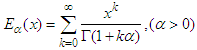as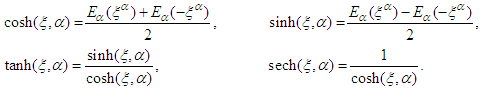

From these definitions, some relations can be obtained [43, 59], firstly, the product of two power series is given by

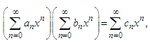(15)

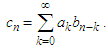where For simplicity, we suppose that

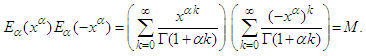To compute the value of by using Eq. (15), the product

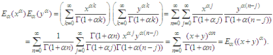This gives that is equal to one.

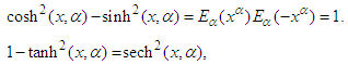Secondly, the fractional derivatives of the Mittag-Leffler function take the form

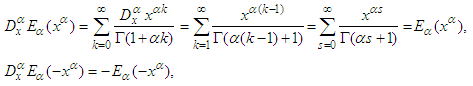The fractional derivatives of the generalized hyperbolic functions take the form

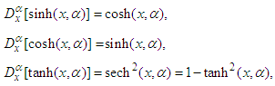where the fractional derivative of is considered as the fractional derivative of division of two functions over (see proposition 2.6 page 732 in [69]). To obtain the fractional derivative of the function it will be considered as times similarly will be considered as times (see proposition 2.4 page 732 in [69]).

Substituting (14) into the FODE (13) and collecting coefficients of equating each coefficient to zero, we obtain a set of algebraic equations of and Solving the algebraic system of equations to obtain Substituting into (14), we have the formal solutions of (11).

4. Space- Time Fractional Quantum Zakharov System

Quantum Zakharov equations are obtained by a quantum fluid approach. These quantum Zakharov equations are applied to two model cases, namely, four-wave interaction and decay instability [57]. In the case of four-wave instability, sufficiently large quantum effects tend to suppress the instability. For decay instability, the quantum Zakharov equations lead to results similar to those of the classical decay instability, except for quantum correction terms in the dispersion relations. Specifically, to obtain the quantum Zakharov equations, they assume a two-species, one-dimensional quantum plasma in the electrostatic approximation. Pressure effects are neglected for the ions whereas the electrons are described by an isothermal equation of state. In contrast to the quantum degenerate case [58], the present model is more suitable for investigating the classical limit . The system takes into account diffraction, which is the most prominent quantum effect, but neglects the quantum statistical effect, dissipation, spin, and relativistic corrections. These effects may be important in more realistic models for small semiconductor devices. Nevertheless, it is useful to consider simplified models that capture the main features of quantum plasmas. Indeed, the present model is sufficiently rich to display a wide variety of behaviors, as will be seen in the rest of this work.

The space-time fractional quantum Zakharov system, which is a transformed generalization of the quantum Zakharov system [38], is defined as follows:

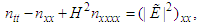
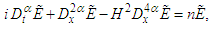(16)

(17)

Since Where is the electric field, is the plasma density, and is the dimensionless quantum parameter

(18)

We restrict the fractional order on the interval that is to keep the spatial fractional derivative term within the interval , i.e. The quantum parameter given in eq. (18) expresses the ratio between the ion plasmon energy and the electron thermal energy. If we set we simply obtain the classical model. At the classical level, a system of nonlinear wave equations describing the interaction between high-frequency Langmuir waves and low-frequency ion-acoustic waves was first derived by Zakharov [59, 60]. Since then, this system has been the subject of a large number of studies [61]. In one dimension, the space-time fractional Zakharov system can be written (in normalized units) as

(19)

(20)

where is the envelope of the high-frequency electric field and n is the plasma density measured from its equilibrium value.

We assume the solution of the space-time quantum Zakharov system (16) and (17) as

(21)

where and are real functions of are positive real unknown constants to be determined. To compute the fractional derivatives in Eqs. (16) and (17), the transformation (21) and Eqs (3, 9 and 10) are used, then we have

(22)

(23)

(24)

Since where equal unity according to the equality contains the function it will be considered as times when the fractional derivative is carried out [62]. Then we have

(25)

(26)

Substituting Eqs (22- 26) in Eqs (16) and (17), we have

(27)

(28)

(29)

Inserting the fractional differential of Eq. (27) in Eq. (28) gives

(30)

To solve Eqs (29) and (30) by using the tanh expansion method, we set

(31)

(32)

By leading order analysis, we obtain thus Eqs (31) and (32) have the form

(33)

Substituting Eq. (33) into Eqs (29) and (30), collecting all terms with the same order of and setting each coefficient of to zero. This yields a system of over-determined algebraic equations for and Solving this system, we can distinguish the following:

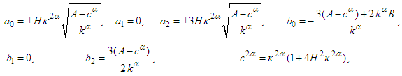(34)

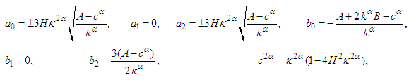(35)

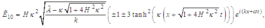
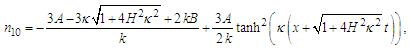
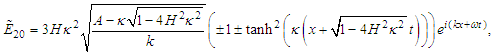
where and The analytical solution of the space-time fractional quantum Zakharov system can be written as

(36)

(37)

(38)

(39)

The solitary wave solutions (36-39), are induced by the fractional order derivative and the quantum parameter H. When is neglected the solitary wave solutions disappear The results provide strong evidence that the terms proportional to and the fractional order derivative in Eqs (36), and (38), modified the dispersion-nonlinearity equilibrium, which is ultimately responsible for the existence of solitons. The square of the amplitude of represents the intensity of a propagating soliton. To understand the effect of the fractional order Eqs (36-39) will be studied as follows. By selecting the values of the parameters and the signs in the Eqs (36) and (38), the bright, gray, and W-solitons can be obtained. The W-soliton is obtained from Eq. (36) by taking this form

(40)

The intensity of W-soliton is graphed as 3-dimensional, versus x and t, in Figure 1. The used parameters are Figure (1-a), the 3-dimensional graph of versus x and t, at . Figure (1-b), the intensity is plotted versus x at constant time with different values of the fractional order derivative From Fig. 1, we can see that, the full width at half maximum (FWHM) of the soliton and the intensity increased when the fractional order value goes up. The gray-soliton is obtained from Eq. (36) by taking this form

(41)

The intensity of gray-soliton is graphed as 3-dimensional, versus x and t, in Figure 2. The used parameters are and Figure (2-a), the 3-dimensional graph of versus x and t, at . Figure (2-b), the intensity is plotted versus x at constant time with different values of the fractional order derivative From Fig. 2, we can see that, the FWHM of the soliton and the intensity increased when the fractional order increased. From Eq. (38) another gray soliton can be obtain by taking the form

(42)

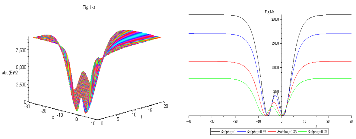Figure (1). Evolutional behavior of given by Eq. (40) of the W-soliton with 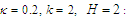(a) Intensity versus x and t at (b) Intensity versus x at and

Figure (2). Evolutional behavior of given by Eq. (41) of the gray soliton with (a) Intensity versus x and t at (b) Intensity versus x at and

The intensity of gray-soliton is graphed as 3-dimensional, versus x and t, in Figure 3. The used parameters are and . Figure (3-a), the 3-dimensional graph of versus x and t, at Figure (3-b), the intensity is plotted versus x at constant time with different values of the fractional order derivative

Also, the bright soliton can be obtained from Eq. (38) by taking the form

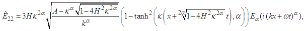(43)

The intensity of bright-soliton is graphed as 3-dimensional, versus x and t, in Figure 4. The used parameters are and Figure (4-a), the 3-dimensional graph of versus x and t, at Figure (4-b), the intensity is plotted versus x at constant time with different values of the fractional order derivative. Figure 4 shows that the increasing of increases the height and the width. Figures 1 to 4 shows that the change of the fractional order derivative affect the soliton behaviors in a fundamental way. Therefore, the fractional derivative can be used to modulate the shape of soliton. Moreover the solitons propagate at phase velocities, and respectively.

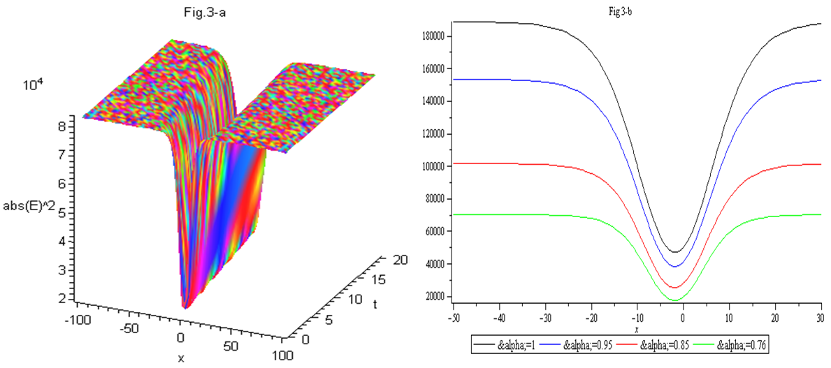Figure (3). Evolutional behavior of given by Eq. (42) of the gray soliton with 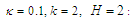(a) Intensity versus x and t at (b) Intensity versus x at and

Figure (4). Evolutional behavior of given by Eq. (43) of the bright soliton with (a) Intensity versus x and t at (b) Intensity versus x at and

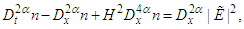
When Eqs (16) and (17) reduce to the well known quantum Zakharov system for plasmas [38, 63]

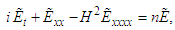(44)

(45)

The solutions (36) - (39) take the form of the following solutions of the quantum Zakharov system for plasmas:

(46)

(47)

(48)

(49)

where and The results obtained by Yang et al [38], El-Wakil and Abdou [63], and Fang Shaomei et al [64] are recovered.

5. Conclusions

The fractional tanh function expansion method is utilized, to construct exact analytical solutions of the space-time fractional quantum Zakharov system for plasmas for the first time. Bright, gray, and W-solitons are investigated. The mathematical software “Maple” is used to plot the obtained results. The changing of the fractional order derivative value and the quantum parameter H affect the solitons behaviors in a fundamental way. To the best of our knowledge, the obtained solutions have not been reported before in the literature. The discussion of the solutions show that the fractional order of the space-time fractional quantum Zakharov system changes both the height and the width of the waves. Therefore, the fractional order can be used to modulate the shape of the waves described by the quantum Zakharov system. Some advantage of this study are as follows: The solutions of the space-time fractional quantum Zakharov system are appeared in closed analytical forms in terms of Mittag-Leffler function. The used technique leads to new solutions describe Bright, gray, and W-solitons that can explain different physical phenomena. Mathematical packages can be used to perform more complicated, elaborate and tedious algebraic calculations.